
6.3 Anchoring
Anchoring means leaning too heavily on the first number you see when you make a later estimate. It is like a price tag that sticks in your mind. In investing, the costliest anchor is your own purchase price, which has no bearing on a stock’s future return.
Why it matters: What you paid is not a reason to hold or to sell.
Summary: Anchoring is leaning too heavily on an initial number when making a later estimate. In investing the costliest anchor is your own purchase price, which has no bearing on a stock’s future return.
- In Tversky and Kahneman’s 1974 experiment, a random wheel number of 10 or 65 moved median estimates from 25 to 45, even with payment for accuracy.
- Nearness to the 52-week high explains a large portion of momentum profits (George and Hwang, 2004).
- A 50% loss needs a 100% gain to recover, about 9 years at 8% a year.
- Use a fresh-cash test: would you buy this holding at today’s price with new money?
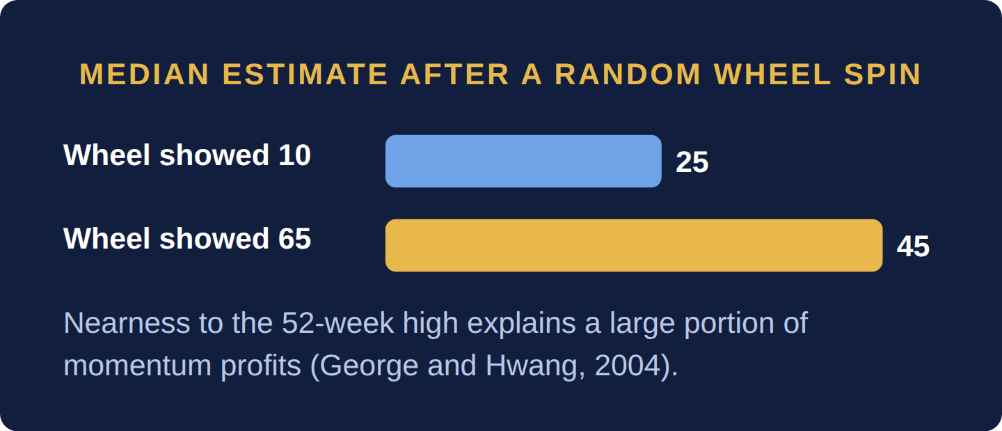
Anchoring is the tendency to rely too heavily on an initial number (the “anchor”) when making a later estimate, even when that number is irrelevant to the question. Tversky and Kahneman’s 1974 demonstration in Science is the classic: subjects watched a wheel of fortune produce a number between 0 and 100, said whether the answer was higher or lower, and then estimated quantities such as the percentage of African countries in the United Nations. The median estimate was 25 for the group that saw 10 and 45 for the group that saw 65, and paying subjects for accuracy did not reduce the effect. Tversky and Kahneman’s explanation is insufficient adjustment: people start from the anchor and move toward the answer, but stop too soon.
In investing, the most expensive anchor is your own purchase price. Holding on until a stock “gets back to what I paid” ties the decision to a number that has no bearing on the stock’s future return; the market does not know or care what you paid. Market-wide anchors matter too. George and Hwang (Journal of Finance, 2004) found that a stock’s nearness to its 52-week high, a number printed on every quote screen, explains a large portion of the profits from momentum investing, consistent with investors anchoring on that price and reacting too slowly to news that should carry the stock past it. Analyst price targets, IPO offer prices and round index levels can act the same way.
A stock bought at $50 now trades at $30. Returning to $50 requires a gain of 50 ÷ 30 − 1 = 66.7%. At an illustrative 8% annual return, that takes ln(1.667) ÷ ln(1.08) ≈ 6.6 years. The required gain grows faster than the loss:
| Decline from purchase price | Gain needed to break even | Years at 8% a year |
|---|---|---|
| 10% | 11.1% | 1.4 |
| 25% | 33.3% | 3.7 |
| 40% | 66.7% | 6.6 |
| 50% | 100.0% | 9.0 |
| 75% | 300.0% | 18.0 |
None of these numbers should drive the decision. The only relevant question is whether the $30 left in this stock has a better expected return, after tax and risk, than $30 invested elsewhere. If it does not, the break-even target is an anchor that costs you the difference every year you wait.
Anchors also shape professional estimates: a valuation that starts from last year’s price target or from the current market price inherits that starting point, which is why careful analysts build their estimate from cash flows before looking at the market (Volume II, Part 1.3: The Actuarial Function — Pricing Risk Before It Happens covers the discounted cash flow model).
Anchoring on a purchase price and the disposition effect (Part 6.7: The Disposition Effect) share one mechanism: an arbitrary historical number, what you paid, becomes the reference point that defines gain and loss. Prospect theory then does the rest. Below the anchor you are in the convex, risk-seeking region of the value function (Part 6.2: Loss Aversion and Prospect Theory), so holding a loser in the hope of getting even feels better than locking in a sure loss, whatever the stock’s prospects.
Apply a “fresh cash” test to every holding at least once a year: if this position’s current value were cash today, would you buy this security at today’s price? If yes, hold; if no, sell or trim, whatever you paid. The one exception is timing for tax: if a gain will turn long-term within a few weeks, waiting can be worth it (Part 6.7: The Disposition Effect). When you must estimate a value, write your own estimate down before you look at a price target, the last price or the 52-week high, then compare. Your purchase price still matters for tax records; it should not matter for the decision.
Waiting to break even on a stock you would not buy today. A position down 50% needs a 100% gain to recover, about 9 years at 8% a year. Suppose, illustratively, the business has deteriorated and the stock’s own expected return is only 3% a year. Leaving $30,000 in it for 9 years grows to $30,000 × 1.039 ≈ $39,143; moving it into a diversified fund expected to earn 8% grows to $30,000 × 1.089 ≈ $59,970. The expected cost of the anchor is about $20,800, before counting the tax deduction you give up by not realizing the loss (Part 6.7: The Disposition Effect).
What is an example of anchoring bias in investing?
The most common example is refusing to sell a stock until it returns to the price you paid. The purchase price is an anchor: it says nothing about the stock’s future return, yet it shapes the decision. Other anchors include the 52-week high, analyst price targets and a stock’s IPO price. Each is a number that is easy to see and hard to ignore, not a measure of value.
How do you avoid anchoring bias?
Form your own estimate before you see any reference number, then compare. For holdings, use a fresh-cash test: would you buy this position at today’s price with new money? Written valuation ranges and asking a colleague to estimate independently also help. Knowing about anchoring does not remove it; in Tversky and Kahneman’s 1974 experiment, paying people for accuracy did not reduce the effect.
Is anchoring the same as the disposition effect?
No, but they are linked. Anchoring is the general tendency to lean on an initial number; the disposition effect is a specific trading pattern, selling winners too early and holding losers too long. The purchase price is the anchor that decides which positions feel like winners and losers, and prospect theory’s value function then pushes you to lock in gains and gamble on losses (Part 6.7: The Disposition Effect).
Anchoring ties estimates to an initial number, and the purchase price is the anchor that costs investors most. Judge each holding by its forward-looking return with a fresh-cash test, and write down your own estimate before looking at targets or past prices.
Six questions on this chapter. Decide on your answer first, then click “Reveal Answer.”
1. You bought a stock at $40 and it now trades at $25. What gain is needed to get back to your purchase price?
- 160%
- 15%
- 37.5%
- 60%
Reveal Answer
Answer: D. 40 ÷ 25 − 1 = 0.60; the 37.5% decline needs a larger percentage gain to recover.
2. Which test does the chapter recommend for deciding whether to keep a holding?
- Would you buy it at today’s price with new money?
- Whether it has returned to your purchase price
- Whether it trades above its own 52-week high price
- Whether analysts’ targets exceed today’s price
Reveal Answer
Answer: A. The fresh-cash test ignores the purchase-price anchor and looks only at forward-looking value.
3. George and Hwang (2004) found that which readily available number explains a large portion of momentum profits?
- The stock’s book value per share
- A stock’s nearness to its 52-week high
- A stock’s distance from its IPO price
- The consensus analyst price target
Reveal Answer
Answer: B. Investors appear to anchor on the 52-week high and react too slowly to news that should carry the price past it.
4. In Tversky and Kahneman’s 1974 wheel-of-fortune experiment, what happened when subjects were paid for accuracy?
- The anchoring effect disappeared completely
- Only the high-anchor group was affected
- The anchoring effect was not reduced
- Estimates moved away from the anchor
Reveal Answer
Answer: C. Payoffs for accuracy did not reduce anchoring, which is why awareness or incentives alone are weak remedies.
5. Worked problem: In an anchoring experiment, median estimates were 25 after a low random number and 45 after a high one. By how much, and what percentage, did the anchor move the estimate?
Reveal Answer
Answer: Difference = 20, or 80% of the low-anchor estimate.
6. Worked problem: A stock’s 52-week high is $80 and it trades at $64. How far below the high is it, and why might investors anchor on it?
Reveal Answer
Answer: 1 − 64 ÷ 80 = 20% below. Investors anchor on the high as a reference point, which affects momentum.
6.4 Overconfidence and Illusion of Control
Overconfidence is thinking your knowledge and forecasts are more accurate than they are. In markets it shows up mainly as trading too much. The cost is large and has been measured: in Barber and Odean’s data, the most active US households lagged the market by 6.5 points a year.
Why it matters: The more you trade on confidence, the more you can give away.
Summary: Overconfidence is overestimating the accuracy of one’s own knowledge and forecasts; in markets it shows up mainly as excessive trading. The cost is large and measured: the most active US households lagged the market by 6.5 points a year in Barber and Odean’s data.
- US CFOs’ 80% forecast ranges contained the realized market return only 36% of the time.
- Men traded 45% more than women, and trading cut their net returns by 2.65 points a year against 1.72.
- In Taiwan, individuals’ aggregate portfolio lost 3.8 points a year to trading, equal to 2.2% of GDP.
- A 2.65-point annual drag turns $100,000 into about $234,000 instead of $387,000 over 20 years at 7%.
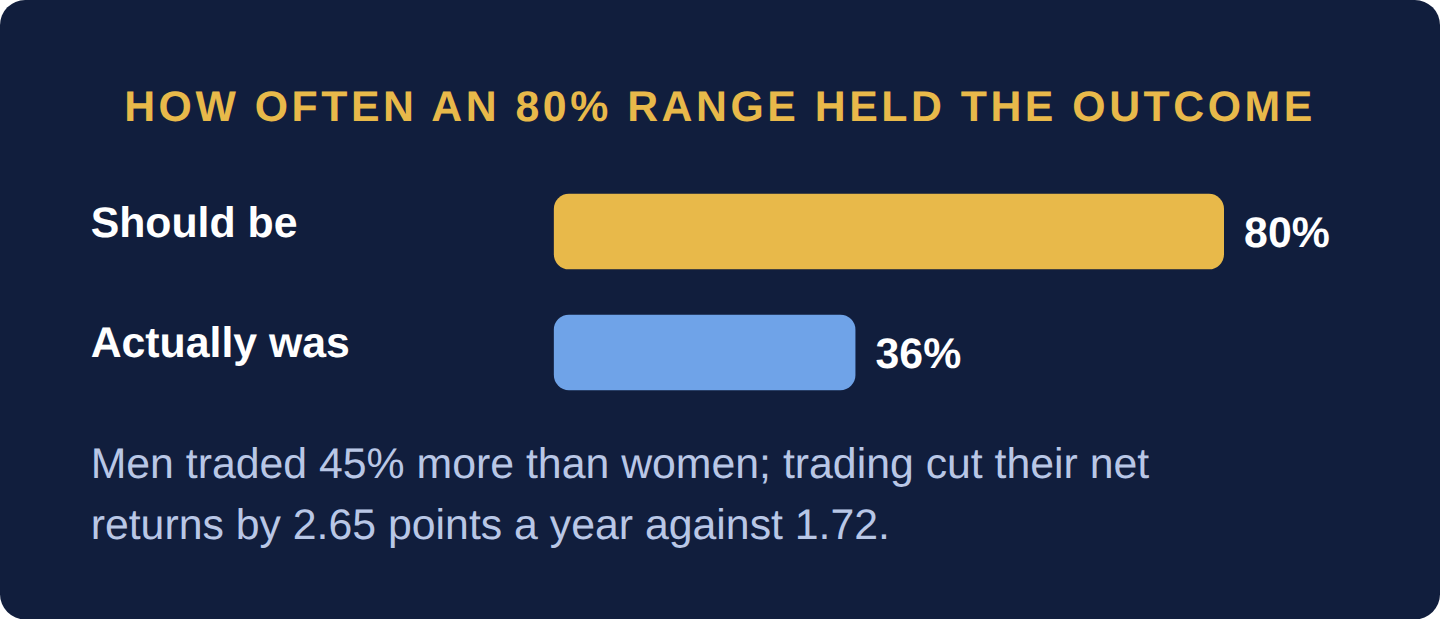
Overconfidence is the consistent tendency to overestimate the accuracy of one’s own knowledge, judgments and forecasts. Its best-measured form is miscalibration, forecast ranges that are too narrow. In a ten-year panel of more than 13,300 stock-market forecasts by US chief financial officers, realized market returns fell inside the executives’ 80% confidence intervals only 36% of the time (Ben-David, Graham and Harvey, Quarterly Journal of Economics, 2013). A related form is the illusion of control, named by psychologist Ellen Langer in 1975: believing one can influence outcomes that are random or largely unpredictable, such as short-term stock price moves.
In markets, overconfidence shows up as excessive trading. Every trade costs commissions, the bid-ask spread (Part 5.3: Market Makers and the Bid-Ask Spread) and often taxes, so trading pays only if the trader knows more than the counterparty. Barber and Odean’s study of 66,465 US households at a discount broker over 1991–1996 found that the average household turned over about 75% of its portfolio a year and earned 16.4% a year against 17.9% for the market; the most active fifth earned 11.4%. A follow-up on more than 35,000 households found that men traded 45% more than women and that trading cut men’s net returns by 2.65 percentage points a year against 1.72 for women, the pattern predicted if men are more overconfident about investing (Barber and Odean, 2001). Using Taiwan Stock Exchange trading data, Barber, Lee, Liu and Odean (2009) estimated that the aggregate portfolio of individual investors lost 3.8 percentage points a year to trading, equivalent to 2.2% of Taiwan’s GDP, while institutions gained 1.5 points.
Assume, illustratively, a $100,000 portfolio and a 7% annual return before trading costs. Buy and hold: $100,000 × 1.0720 ≈ $386,968. With the 2.65-point drag measured for men: $100,000 × 1.043520 ≈ $234,341. With the 1.72-point drag measured for women: $100,000 × 1.052820 ≈ $279,845. The higher-turnover investor ends about $152,600 behind the buy-and-hold investor, 39% of the passive outcome, with the same assets and the same gross return.
The bias is not cured by intelligence or information. It is managed by measurement: a written record of forecasts and their stated confidence, scored against what happened, is the only reliable way to discover whether your confidence is earned.
Overconfidence is documented among professionals, not only retail investors: the CFOs in the miscalibration study are among the best-informed forecasters in the economy, yet their 80% ranges caught the outcome barely a third of the time. Expertise does not remove the bias, which is why firms rely on process controls: independent review of significant decisions (the maker-checker principle in Volume I’s Part 8), position and loss limits, and pre-mortems in which a team assumes a decision has failed and explains why. If you work in an investment role, keeping a forecast log with stated confidence levels, scored each year, is a credible way to show judgment that is calibrated rather than merely confident.
Set a turnover budget and make each discretionary trade justify itself. Before trading, write down the expected gain, why the counterparty is wrong, and the all-in cost (spread, commission, tax). If you cannot name the counterparty’s mistake, or the expected gain is not several times the cost, do not trade. As a rough guide, annual turnover above about 50% in a personal long-term portfolio deserves a written justification. Ignore the budget for rebalancing to target weights and for tax-loss harvesting, which are rule-driven, not forecast-driven.
Trading on conviction instead of measured edge. The cost compounds out of sight: the example above turns a 2.65-point annual drag into a $152,600 shortfall on $100,000 over 20 years, and nothing on a monthly statement shows the portfolio you would have had. Keep a log of every discretionary trade and compare it once a year with simply having held. If the log shows no edge after costs, it has paid for itself.
What is overconfidence bias in investing?
It is overestimating how accurate your knowledge and forecasts are. In investing it shows up as forecast ranges that are too narrow, belief that you can time short-term moves, and above all excessive trading. In Barber and Odean’s data on 66,465 US households over 1991–1996, the most active fifth earned 11.4% a year while the market returned 17.9%.
Does trading more lead to lower returns?
On average, yes, for individual investors. Each trade costs spread, commission and often tax, and the counterparty is often a better-informed professional. Barber and Odean found the heaviest traders earned the least, and in Taiwan the aggregate portfolio of individuals lost 3.8 percentage points a year to trading. Low turnover does not guarantee good returns; high turnover has a measurable average cost.
What is the illusion of control?
The illusion of control is the belief that you can influence outcomes that are mostly random. Psychologist Ellen Langer named and tested it in a 1975 paper. In investing it appears as the belief that watching screens closely, or choosing the perfect entry point, gives control over short-term price moves that are largely unpredictable.
Are professional fund managers overconfident too?
Yes. Overconfidence is documented in professionals, including US CFOs whose 80% stock-market forecast ranges contained the outcome only 36% of the time over a decade. Experience improves knowledge but not necessarily calibration, which is why investment firms use independent review, risk limits and forecast logs instead of relying on individual judgment.
Overconfidence shows up as forecast ranges that are too narrow and as excessive trading, which cost the most active US households 6.5 points a year against the market in 1991–1996. Professionals are not exempt, so the remedy is measurement and process: turnover budgets, written trade rationales and forecast logs.
Six questions on this chapter. Decide on your answer first, then click “Reveal Answer.”
1. Over a decade of surveys, how often did realized market returns fall inside US CFOs’ 80% confidence intervals?
- 64% of the time
- 52% of the time
- 80% of the time
- 36% of the time
Reveal Answer
Answer: D. Ben-David, Graham and Harvey (2013) found intervals far too narrow: 36% coverage against 80% intended.
2. A $50,000 portfolio earns 6% a year before trading costs. Over 15 years, about how much does a 2-point annual trading drag cost?
- About $36,400
- About $29,800
- About $15,000
- About $20,600
Reveal Answer
Answer: B. $50,000 × 1.0615 ≈ $119,828 versus $50,000 × 1.0415 ≈ $90,047, a gap of about $29,800.
3. In Barber and Odean’s 2001 study of more than 35,000 households, how did men’s trading compare with women’s?
- Men traded 45% more and lost more return to trading
- Men traded more but earned higher net returns
- Men and women traded equally but men chose riskier stocks
- Women traded 45% more and lost more return to trading
Reveal Answer
Answer: A. Trading cut men’s net returns by 2.65 points a year against 1.72 for women, consistent with greater overconfidence.
4. An investor believes watching price screens all day lets her time short-term moves in a stock. Which bias does this best illustrate?
- Disposition effect
- Mental accounting
- Illusion of control
- Informational cascade
Reveal Answer
Answer: C. The illusion of control is believing one can influence or foresee outcomes that are largely random, such as short-term price moves.
5. Worked problem: CFOs’ 80% forecast ranges contained the realized return only 36% of the time. By how many percentage points were they overconfident?
Reveal Answer
Answer: 80% − 36% = 44 percentage points.
6. Worked problem: Trading cut net returns by 2.65 points a year for men and 1.72 for women, from a gross 8%. What would $100,000 grow to over 20 years for each?
Reveal Answer
Answer: Men: net 5.35%: $283,590. Women: net 6.28%: $338,089. The difference is $54,499.
- Tversky & Kahneman (1974), Judgment under Uncertainty: Heuristics and Biases, Science — The classic anchoring experiments