
6.1 Challenging the Rational Actor
Classical finance assumes investors are rational: they weigh outcomes carefully and maximize expected utility. Behavioral finance documents the ways real people systematically and predictably depart from that. Normally, mistakes would cancel out, since some people err one way and some the other. But the errors are often correlated across people, and betting against them is costly, so some of them reach market prices.
Why it matters: Mistakes only move prices when many people make the same one.
Summary: Behavioral finance documents systematic, predictable ways real investors depart from the rational, expected-utility maximizer assumed by Modern Portfolio Theory and CAPM. Because the errors are correlated across people and arbitrage is costly, some of them reach market prices instead of canceling out.
- Kahneman (2002) and Thaler (2017) received Nobel Prizes for bringing psychology into economics.
- Errors move prices only when they are correlated across investors and the limits to arbitrage stop professionals from correcting them.
- Grade any behavioral claim on three rungs: the lab, real-money accounts, and market prices; the evidence thins as you climb.
- The same research shows who pays: the most active US households earned 11.4% a year against 17.9% for the market in 1991–1996.

Modern Portfolio Theory (Part 5.2 of Volume II) and the Capital Asset Pricing Model, CAPM (Part 1.5 of Volume II), both rest on the assumption of a rational actor: an investor who processes information without systematic error, holds stable preferences and chooses as if maximizing expected utility, the probability-weighted average of how much each possible level of final wealth is worth to them. Beginning with the work of psychologists Daniel Kahneman and Amos Tversky in the 1970s, behavioral finance has documented, first in experiments and later in millions of brokerage records, systematic and predictable ways real investors depart from that assumption. Kahneman shared the 2002 Nobel Prize in economic sciences “for having integrated insights from psychological research into economic science,” and Richard Thaler, who carried the ideas into finance, received the 2017 prize for contributions to behavioral economics. The deviations are not random noise that cancels out across a large population; they are directional, shared by many people at once, and in some settings strong enough to move prices.
Why do errors that each individual makes fail to wash out in the aggregate? Two reasons. First, the errors are correlated: people use the same mental shortcuts (heuristics) and react to the same headlines, so millions of small mistakes point the same way instead of offsetting. Second, the professionals who could profit by trading against those mistakes face costs and risks that cap how much they will bet, the limits to arbitrage covered in Part 6.8: What This Means for Markets and Individual Investors. A bias that is correlated across investors and expensive to arbitrage can show up in prices; one that is random, or cheap to trade against, cannot.
Every claim in this Part can be graded on three rungs, and the evidence gets thinner as you climb.
- Rung 1, the lab: does the pattern appear in controlled choices? Prospect theory’s core patterns pass easily: a 2020 replication with 4,098 participants in 19 countries and 13 languages reproduced 94% of the original 1979 items, with some attenuation (Ruggeri and colleagues, Nature Human Behaviour).
- Rung 2, real money: does it survive when people trade their own savings? Excessive trading (Part 6.4: Overconfidence and Illusion of Control) and the disposition effect (Part 6.7: The Disposition Effect) pass: the first was measured in the records of 66,465 US brokerage households, the second in 10,000 US brokerage accounts.
- Rung 3, prices: does it move market prices after arbitrage? This is the hardest and most contested rung. It needs correlated errors and limits to arbitrage at the same time (Part 6.8: What This Means for Markets and Individual Investors).
A finding on rung 1 tells you about people. Only a finding on rung 3 tells you something about the market you trade in, and even then it says nothing about whether you, after costs, can profit from it.
The rest of this Part works through the patterns with the strongest evidence: how gains and losses are valued (Part 6.2: Loss Aversion and Prospect Theory), anchors (Part 6.3: Anchoring), overconfidence (Part 6.4: Overconfidence and Illusion of Control), herding (Part 6.5: Herding Behavior), mental accounting and defaults (Part 6.6: Mental Accounting), the disposition effect (Part 6.7: The Disposition Effect), and what all of it means for prices and for your own decisions (Part 6.8: What This Means for Markets and Individual Investors).
This is a reading rule. Before acting on any behavioral finding, ask which rung it has cleared. If it has only laboratory evidence, use it to design your own process (defaults, checklists, cooling-off periods), never as a trading signal. If it has field evidence that individuals like you lose money from it, change your own behavior first, because that saving is certain. Treat a claimed price anomaly as tradable only if you can say who is on the other side, why arbitrageurs have not removed it, and what it costs you to hold the position until it closes. Ignore the rule for purely descriptive questions, where laboratory evidence is enough.
Reading “markets are not perfectly rational” as “so I can beat them by trading.” The research that documents investor biases also documents who pays for them. In Barber and Odean’s study of 66,465 US households at a discount broker over 1991–1996, the fifth of households that traded most earned 11.4% a year while the market returned 17.9%. On $100,000 over those six years: $100,000 × 1.1146 ≈ $191,122 for the active traders against $100,000 × 1.1796 ≈ $268,586 for the market, a shortfall of about $77,500. The investor most exposed to biases is the one who believes they belong to other people.
What is behavioral finance in simple terms?
Behavioral finance studies how predictable psychological patterns, such as feeling losses more than gains or leaning on irrelevant numbers, shape investors’ decisions and, through them, market prices. It keeps the tools of standard finance (risk, return, diversification) but replaces the assumption that every investor is a flawless calculator with evidence on how people actually choose. Its founding paper is Kahneman and Tversky’s prospect theory of 1979.
Does behavioral finance prove the efficient market hypothesis wrong?
No. It shows that investors make systematic errors and that arbitrage cannot always correct the resulting prices, which weakens the strongest version of market efficiency. It does not show that mispricings are easy to find or to profit from; active traders as a group still lag the market after costs. Many economists hold both views at once: prices can be wrong and still be hard to beat (Part 6.8: What This Means for Markets and Individual Investors).
Is it irrational to be risk averse?
No. Preferring a sure amount to a gamble with the same expected value is fully consistent with expected-utility theory when the stakes are large relative to your wealth. Behavioral finance targets patterns that rational theory cannot explain, such as refusing small favorable bets or reversing a choice when the same outcome is described differently (Part 6.2: Loss Aversion and Prospect Theory).
Who are the founders of behavioral finance?
Psychologists Daniel Kahneman and Amos Tversky laid the foundations with their 1974 work on judgment heuristics and their 1979 prospect theory; Kahneman shared the 2002 Nobel Prize in economic sciences. Economist Richard Thaler carried the ideas into finance and economics, with work on mental accounting and retirement-saving design, and received the 2017 prize for his contributions to behavioral economics.
Behavioral finance shows that investors depart from the rational-actor model in systematic ways, and that correlated errors plus the limits to arbitrage can carry those errors into prices. Grade each claim by whether it holds in the lab, in real accounts and in prices, and remember that the same research shows active traders paying for the biases.
Six questions on this chapter. Decide on your answer first, then click “Reveal Answer.”
1. Why can individual investors’ psychological errors affect market prices instead of canceling out across millions of people?
- Their errors are correlated, and trading against them is costly
- Each investor’s errors are too large for other investors to offset
- Regulators prevent professionals from trading against retail investors
- Prices are set by retail investors alone, not by professionals
Reveal Answer
Answer: A. Errors that point the same way do not offset, and the limits to arbitrage cap how much professionals will bet against them.
2. Using Barber and Odean’s figures (11.4% a year for the most active fifth vs 17.9% for the market, 1991–1996), about how far behind would $100,000 fall over the six years?
- About $65,000
- About $77,500
- About $91,000
- About $39,000
Reveal Answer
Answer: B. $100,000 × 1.1796 ≈ $268,586 and $100,000 × 1.1146 ≈ $191,122; the gap is about $77,500 (simple 6.5 × 6 points would understate it at $39,000).
3. In the chapter’s three rungs of evidence, which claim is the hardest to establish?
- That a bias appears in survey answers about money
- That a bias appears in controlled laboratory choices
- That a bias appears in real brokerage account records
- That a bias moves market prices after arbitrage
Reveal Answer
Answer: D. The price rung needs both correlated errors and binding limits to arbitrage, and it is the most contested.
4. A bias is documented only in laboratory experiments. Under the chapter’s reading rule, what is its best use?
- Treating it as proof that market prices are wrong
- Dismissing it, because laboratory evidence has no value
- Designing your own process, such as defaults or checklists
- Trading against other investors who are likely to show this bias
Reveal Answer
Answer: C. Lab-only findings describe people, not prices, so they guide personal process design, never trading signals.
5. Worked problem: A gamble pays +$150 or −$100 with equal probability. What is its expected value, and its prospect-theory value with a loss-aversion coefficient of 2.25 (linear for simplicity)?
Reveal Answer
Answer: EV = 0.5 × 150 + 0.5 × (−100) = +$25. Prospect value = 0.5 × 150 − 0.5 × 2.25 × 100 = -37.5, so the loss-averse investor refuses.
6. Worked problem: What payoff on the win would make a loss-averse investor (2.25) indifferent to a 50/50 bet that loses $100?
Reveal Answer
Answer: Win = 2.25 × $100 = $225.
6.2 Loss Aversion and Prospect Theory
Prospect theory says people judge gains and losses from a reference point, not from the final total. Losses hurt about twice as strongly as equal gains please, and people overweight rare events. Refusing a big fair bet only shows risk aversion. Refusing a small bet in your favor, or reversing a choice just because the reference point moved, is the signature of loss aversion.
Why it matters: A loss feels bigger than an equal gain, and that changes real decisions.
Summary: Prospect theory says people value gains and losses from a reference point, feel losses about twice as strongly as equal gains, and overweight rare events. Refusing a large fair bet only shows risk aversion; refusing a small favorable bet, or reversing a choice when only the reference point moves, is the signature of loss aversion.
- Tversky and Kahneman’s 1992 fit: v(x) = x0.88 for gains, −2.25 × (−x)0.88 for losses; a 2024 meta-analysis puts the mean coefficient at 1.955.
- A rational household with $250,000 would pay about $20,900 to avoid a ±$100,000 coin flip, so refusing it proves nothing about loss aversion.
- With the 1992 parameters a 50/50 bet that loses $100 needs a win of about $274 to be accepted; the rational benchmark needs about $100.
- Decision weights turn a 1% chance into about 4% (losses) and a 0.1% chance into about 1.45% (gains), which sells both insurance and lottery tickets.
- The direction replicates in 19 countries; the size, and some classic demonstrations, are debated.
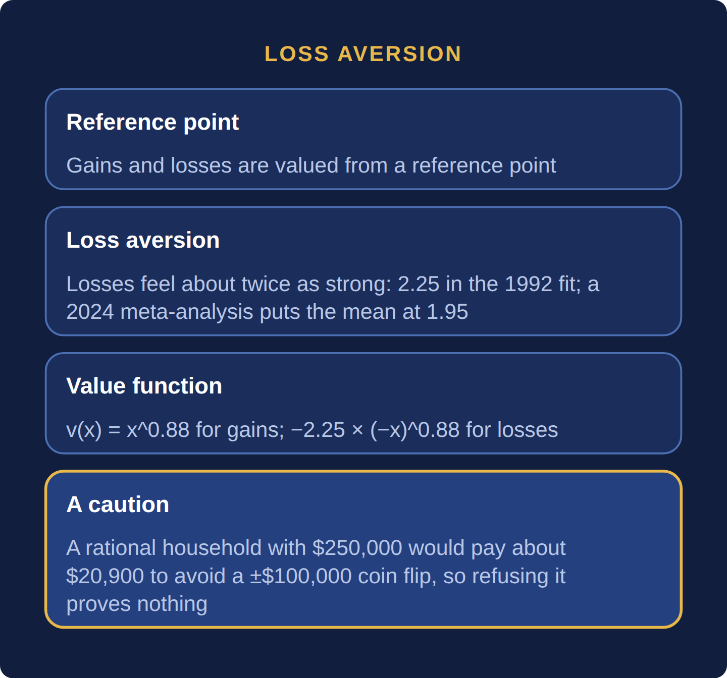
Kahneman and Tversky’s Prospect Theory (1979) changed what people are assumed to evaluate. Standard theory scores each option by the final wealth it produces. Prospect theory scores it by the change from a reference point, usually the status quo, a purchase price or an expectation, and treats changes below that point differently from changes above it. The central asymmetry is loss aversion: a loss hurts more than an equal gain pleases. In Tversky and Kahneman’s 1992 estimates the loss-aversion coefficient, the ratio of the pain of losing a dollar to the pleasure of gaining one, was 2.25. Standard portfolio theory has no such kink.
The value function has three features. It is concave for gains, which makes people cautious among gains; convex for losses, which makes people gamble to avoid a sure loss, the engine of the disposition effect (Part 6.7: The Disposition Effect); and kinked at the reference point, where losses are steeper than gains. Move the reference point and the same final wealth can be coded as a gain or as a loss, which is why the way a choice is framed can reverse it.
Tversky and Kahneman’s 1992 cumulative prospect theory fits v(x) = x0.88 for gains and v(x) = −2.25 × (−x)0.88 for losses. Substituting: v(+$100) ≈ 57.5 and v(−$100) ≈ −129.5; v(+$1,000) ≈ 436.5 and v(−$1,000) ≈ −982.2. Ten times the money produces only about 7.6 times the feeling (436.5 ÷ 57.5), the concavity, and every loss weighs 2.25 times its matching gain, the kink.
Probabilities are replaced by decision weights, w(p) = pγ ÷ (pγ + (1 − p)γ)1/γ, with γ = 0.61 for gains and 0.69 for losses:
| Probability | Weight if a gain | Weight if a loss |
|---|---|---|
| 0.1% | 1.45% | 0.84% |
| 1% | 5.53% | 3.97% |
| 50% | 42.1% | 45.4% |
| 99% | 91.2% | 94.5% |
Rare events are overweighted and likely ones underweighted, which produces the fourfold pattern: risk aversion for likely gains and unlikely losses, risk seeking for likely losses and unlikely gains.
The classic illustration, a refused coin flip for large stakes, does not isolate loss aversion, as the worked example shows.
Step 1: a large fair bet does not discriminate. Most people refuse a 50/50 flip to win or lose $100,000, but ordinary risk aversion predicts that too. Take a rational household with $250,000 and logarithmic utility. Its certainty equivalent, the sure amount it values the same as the bet, is √(350,000 × 150,000) − 250,000 ≈ −$20,871: a fully rational investor would pay about $20,900 to avoid this bet.
Step 2: shrink the stakes. Offer 50/50 to win $110 or lose $100. The same household’s certainty equivalent is √(250,110 × 249,900) − 250,000 ≈ +$4.98, almost the bet’s $5 expected value, so expected-utility theory says take it. Most people still refuse. Matthew Rabin (Econometrica, 2000) proved that an expected-utility maximizer who turned down this bet at every wealth level would also have to turn down a 50/50 bet to lose $1,000 or gain any sum at all, which nobody believes. Loss aversion explains the refusal without that absurdity.
Step 3: hold final wealth fixed and move the reference point. Kahneman and Tversky’s 1979 Problems 11 and 12, posed in Israeli pounds and restated here in dollars: Group 1 is given $1,000 and chooses (A) a 50% chance of another $1,000 or (B) a sure $500. Group 2 is given $2,000 and chooses (C) a 50% chance of losing $1,000 or (D) a sure loss of $500. A and C end at $1,000 or $2,000 with equal odds; B and D at a sure $1,500. Final-wealth theory predicts the same choice in both groups; instead 84% of Group 1 (70 respondents) took the sure gain and 69% of Group 2 (68 respondents) took the gamble.
| Option | Final wealth | Prospect-theory value | Predicted choice |
|---|---|---|---|
| A: 50% chance of +$1,000 | $1,000 or $2,000 | 0.421 × 436.5 ≈ 183.8 | — |
| B: sure +$500 | $1,500 | 5000.88 ≈ 237.2 | B, the sure gain |
| C: 50% chance of −$1,000 | $1,000 or $2,000 | 0.454 × (−982.2) ≈ −445.9 | C, the gamble |
| D: sure −$500 | $1,500 | −2.25 × 5000.88 ≈ −533.7 | — |
That reversal, not the refusal of a large fair bet, is the signature of reference dependence. (The rupee version of the old example is corrected in the India Lens at the end of this Part.)
Decision weights explain why the same person buys insurance and lottery tickets, both priced above their expected payouts. A household facing a 1% chance of an uninsured $50,000 loss (expected loss $500) is quoted a $600 premium. Uninsured, its prospect-theory value is 0.0397 × (−2.25 × 50,0000.88) ≈ −1,218; insured, −2.25 × 6000.88 ≈ −627. It buys, and would pay up to about $1,277. The insurer’s loading for expenses and profit (Part 1.3: The Actuarial Function — Pricing Risk Before It Happens) is easier to sell because the rare loss is weighted about four times its true probability. The same overweighting makes a $2 ticket with a 1-in-1,000 chance of $1,000, expected value −$1.00, score positive: 0.0145 × 9980.88 − 0.988 × 2.25 × 20.88 ≈ 6.3 − 4.1 = +2.2.
A 50/50 bet loses $100 on tails. What heads payoff G makes each chooser accept? The log-utility household needs G ≥ 100 × 250,000 ÷ 249,900 ≈ $100.04. The prospect-theory chooser needs 0.421 × G0.88 ≥ 0.454 × 2.25 × 1000.88, so G* = 100 × (2.25 × 0.454 ÷ 0.421)1/0.88 ≈ $274.
| Payoff if heads | Expected value | Log-utility certainty equivalent | Prospect-theory value |
|---|---|---|---|
| $110 | +$5.00 | +$4.98: accept | −32.5: reject |
| $200 | +$50.00 | +$49.96: accept | −14.2: reject |
| $300 | +$100.00 | +$99.92: accept | +4.9: accept |
Flip point: the loss-averse chooser needs a win of about $274, 2.74 times the loss; the rational benchmark accepts anything above about $100. Every small favorable risk between the two is one that loss aversion refuses.
How wide that gap is, across people and settings, is debated.
The skeptical case. David Gal and Derek Rucker (Journal of Consumer Psychology, 2018) conclude that the evidence does not show losses, on balance, to be more impactful than gains, and that many classic demonstrations, such as refusing to trade a mug just received, reflect inertia, a preference for inaction.
The replication evidence. A 2020 replication of the 1979 problems with 4,098 participants in 19 countries (Ruggeri and colleagues, Nature Human Behaviour) reproduced 94% of the items, with some attenuation. A 2024 meta-analysis in the Journal of Economic Literature (Brown, Imai, Vieider and Camerer) pooled 607 estimates from 150 articles and found a mean loss-aversion coefficient of 1.955, 95% credible interval 1.820 to 2.102: below 2.25, clearly above 1.
What to take from it. The direction replicates; the size varies. Treat “about two” as a central estimate.
Restate each option as final wealth. If your preference reverses when the same outcome is described as a gain rather than an avoided loss, the frame is choosing, not the economics. As a heuristic, if a risk is under about 1% of your net worth and you will face it many times (deductibles, warranties, ordinary portfolio swings), pick the option with the better expected value. Ignore it for risks large relative to your wealth, where risk aversion is rational.
Paying to avoid small losses you could absorb. Illustratively, cutting a car-insurance deductible from $1,000 to $500 costs $150 a year and you claim once a decade. The extra coverage pays at most $500 per claim, an expected $500 × 0.1 = $50 a year, against $150: an expected loss of $100 a year, about $1,000 a decade on one policy. Keep insurance for losses you cannot absorb (Part 1.1: Why Insurance Exists — Risk Pooling and the Law of Large Numbers).
What is loss aversion in simple terms?
Loss aversion is the tendency to feel a loss more strongly than a gain of the same size. Tversky and Kahneman’s 1992 estimate put the ratio at 2.25; a 2024 meta-analysis found a mean of about 1.96. Losing $100 feels roughly as bad as winning $200 feels good, measured from a reference point such as what you paid.
What is the difference between loss aversion and risk aversion?
Risk aversion is preferring a sure amount to a gamble with the same expected value, explained by the diminishing value of extra wealth. Loss aversion is a kink at a reference point. It shows at small stakes: a rational household with $250,000 accepts a 50/50 bet to win $110 or lose $100; a loss-averse person refuses.
Why do people buy both insurance and lottery tickets?
Because people overweight small probabilities. Under Tversky and Kahneman’s 1992 weighting function a 1% chance of a loss feels like about 4% and a 0.1% chance of a gain like about 1.45%, so a rare disaster looks worth insuring and a rare jackpot worth buying, though both are priced above their expected value.
Prospect theory values changes from a reference point, with losses weighted about two times gains and rare events overweighted. Refusing a large fair bet is ordinary risk aversion; refusing a small favorable one, or reversing a choice when only the reference point moves, is loss aversion, whose size is still debated even though its direction replicates.
Six questions on this chapter. Decide on your answer first, then click “Reveal Answer.”
1. A household with $250,000 refuses a 50/50 bet to win or lose $100,000. What does the refusal show?
- Probability weighting, because 50% is underweighted
- Ordinary risk aversion, also predicted by expected utility
- Anchoring on the large size of the stake being offered
- Loss aversion, because the expected value is exactly zero
Reveal Answer
Answer: B. With log utility the certainty equivalent is about −$20,871, so a fully rational investor refuses too; large fair bets do not isolate loss aversion.
2. Using the 1992 parameters (α = 0.88, λ = 2.25, decision weights 0.421 for a 50% gain and 0.454 for a 50% loss), what heads payoff makes a 50/50 bet that loses $100 just acceptable?
- About $251
- About $225
- About $274
- About $100
Reveal Answer
Answer: C. G* = 100 × (2.25 × 0.454 ÷ 0.421)1/0.88 ≈ $274; $251 ignores probability weighting and $100 is the rational benchmark.
3. Group 1, given $1,000, mostly takes a sure +$500; Group 2, given $2,000, mostly gambles on a 50% chance of −$1,000 over a sure −$500. Final outcomes are identical. What does this reversal demonstrate?
- Reference dependence in coding gains and losses
- Mental accounting of the initial gift as house money
- Overconfidence about the odds of the gamble
- Risk aversion that rises with total wealth
Reveal Answer
Answer: A. Both groups face the same final wealth distribution; only the reference point differs, which flips risk aversion to risk seeking.
4. What mean loss-aversion coefficient did the 2024 Journal of Economic Literature meta-analysis of 607 estimates find?
- About 1.20
- About 3.00
- About 2.25
- About 1.96
Reveal Answer
Answer: D. Brown, Imai, Vieider and Camerer found 1.955 (credible interval 1.820–2.102), below the 1992 estimate of 2.25 but clearly above 1.
5. Worked problem: Using v(x) = x0.88 for gains and −2.25 × (−x)0.88 for losses, what are the values of a $100 gain and a $100 loss?
Reveal Answer
Answer: Gain: 1000.88 = 57.5. Loss: −2.25 × 57.5 = -129.5.
6. Worked problem: A 50/50 bet wins $100 or loses $100. What is its prospect-theory value, and would a loss-averse investor accept it?
Reveal Answer
Answer: Value = 0.5 × 57.5 + 0.5 × (-129.5) = -36.0, negative, so it is rejected even though its expected dollar value is zero.
- Kahneman & Tversky (1979), Prospect Theory: An Analysis of Decision under Risk, Econometrica — The paper that founded prospect theory
- Tversky & Kahneman (1974), Judgment under Uncertainty: Heuristics and Biases, Science — The paper that catalogued heuristics and biases
- Tversky & Kahneman (1992), Advances in prospect theory: Cumulative representation of uncertainty, Journal of Risk and Uncertainty — The cumulative version of prospect theory