
5.5 Algorithmic Execution Strategies
Execution algorithms split a large order into many small pieces so that buying or selling doesn’t push the price against you, which is called market impact. The right way to measure the cost is implementation shortfall: the gap between a paper portfolio traded at the decision price and the real one. Which algorithm to use depends on how fast you expect the price to drift against you while you trade.
Why it matters: A good trade is judged against the price when you decided, not the price when you finished.
Summary: Execution algorithms split large orders to limit market impact, and the right measure of their cost is implementation shortfall: the gap between a paper portfolio traded at the decision price and the real one. The choice of algorithm turns on how fast you expect the price to drift against you.
- Implementation shortfall = delay cost + execution cost + opportunity cost + fees.
- In the worked $10 million order, shortfall was $54,400 (54.4 bps) even though the trader beat VWAP by $11,200.
- Trading slowly cuts impact but adds drift exposure and risk; the Almgren–Chriss framework formalizes the trade-off.
- In the scenario comparison, a three-day schedule wins below 8 bps a day of expected drift and a two-hour burst only above about 58.
- Judging execution by VWAP alone rewards leaving orders unfinished.

A large institutional order — say, a pension fund needing to buy 200,000 shares, or $10 million, of a single stock — cannot simply be sent to the market at once without severely moving the price against the buyer (known as market impact). Execution algorithms exist specifically to break large orders into many smaller pieces, traded strategically over time to minimize this impact.
To choose among algorithms you need a measure of cost. The standard one is implementation shortfall, introduced by André Perold in 1988 (“The Implementation Shortfall: Paper Versus Reality,” Journal of Portfolio Management): the difference between the return of a “paper” portfolio that trades instantly at the price when the decision was made and the return of the real portfolio. Practitioners split it into four parts. Delay cost is the price move between the decision and the moment the order reaches the market. Execution cost is the gap between the arrival price and the average fill price, which captures spread and market impact. Opportunity cost is the move on shares never bought or sold. Fees are commissions and exchange charges. Implementation shortfall counts what most benchmarks miss: the cost of trading slowly and of not finishing.
| Algorithm | Strategy |
|---|---|
| VWAP (Volume-Weighted Average Price) | Splits the order to trade roughly in proportion to the security’s typical historical trading volume pattern throughout the day, aiming to match (not beat) the day’s volume-weighted average price |
| TWAP (Time-Weighted Average Price) | Splits the order into equal-sized pieces traded at even time intervals throughout a specified period, regardless of actual volume patterns |
| Implementation Shortfall | Minimizes expected implementation shortfall by balancing market impact (trading too fast) against timing risk (trading too slowly while the price drifts away), speeding up or slowing down as prices and volume change |
A portfolio manager decides to buy 200,000 shares when the midpoint is $50.00; the paper portfolio is 200,000 × $50.00 = $10,000,000. The order reaches the trader when the midpoint is $50.06. The algorithm buys 160,000 shares at an average of $50.18 and stops; the stock closes at $50.60. Commission is $0.01 a share (an illustrative rate). One basis point of the paper portfolio is $1,000.
| Component | Formula | Cost | bps |
|---|---|---|---|
| Delay | (50.06 − 50.00) × 160,000 | $9,600 | 9.6 |
| Execution | (50.18 − 50.06) × 160,000 | $19,200 | 19.2 |
| Opportunity | (50.60 − 50.00) × 40,000 | $24,000 | 24.0 |
| Fees | 0.01 × 160,000 | $1,600 | 1.6 |
| Total | $54,400 | 54.4 |
Check: the paper portfolio gains (50.60 − 50.00) × 200,000 = $120,000; the real one gains (50.60 − 50.18) × 160,000 − 1,600 = $65,600. The difference, $54,400, is the shortfall. Now suppose the day’s VWAP was $50.25. Against VWAP, the trader bought (50.25 − 50.18) × 160,000 = $11,200 better than the benchmark, about 14 bps, and looks skilled. Against the decision, the trade cost 54.4 bps, and the largest single item was the 40,000 shares never bought.
The core trade-off, formalized by Almgren and Chriss (Journal of Risk, Winter 2000), is between market impact, which falls as you trade more slowly, and timing risk, which rises because the price can drift while the order is unfinished. If you expect the price to drift against you (because your own research is shared by others, or the order is already leaking), slow trading becomes expensive. The comparison below puts numbers on that.
The same 200,000-share buy is 10% of the stock’s average daily volume; daily volatility is 2%. Impact costs are illustrative assumptions in line with the idea that faster trading pays more impact. Let d be the expected adverse drift in bps per day. With a steady schedule over T days, the order is on average half unfilled, so expected drift cost = d × T ÷ 2, and the standard deviation of the cost is about volatility × √(T ÷ 3).
| Scenario | Participation | Impact (bps) | Cost if d = 0 | Cost if d = 30 | Risk (sd, bps) |
|---|---|---|---|---|---|
| A: 2 hours (T = 2 ÷ 6.5 day) | 32.5% | 35 | 35.0 | 35 + 30 × 0.154 = 39.6 | 64 |
| B: full-day VWAP (T = 1) | 10% | 15 | 15.0 | 15 + 30 × 0.5 = 30.0 | 115 |
| C: 3 days (T = 3) | 3.3% | 7 | 7.0 | 7 + 30 × 1.5 = 52.0 | 200 |
Break-even drift between B and C: 15 + 0.5d = 7 + 1.5d, so d = 8 ÷ 1.0 = 8 bps a day. Between A and B: 35 + 0.154d = 15 + 0.5d, so d = 20 ÷ 0.346 ≈ 58 bps a day. With no view, trade patiently (C); with a modest expected drift of 8 to 58 bps a day, the full-day schedule wins; only with strong, fast-decaying information is the two-hour burst worth its impact. On a $10 million order, each basis point is $1,000, so choosing C when drift is 30 bps a day costs (52 − 30) × $1,000 = $22,000 more than B.
The choice of execution algorithm is itself a genuine trading decision with real cost consequences — a trader convinced a stock is about to move sharply against the unfilled part of the order (up for a buyer, down for a seller) will typically choose a more aggressive strategy prioritizing speed over minimizing market impact, while a trader with no strong near-term view will typically default to VWAP specifically to avoid being measured unfavorably against the day’s average price by their own performance-measurement desk.
Measure every order against the price at the moment of decision (implementation shortfall), not VWAP. Then set the pace from expected drift: below about 8 bps a day of adverse drift, spread the order over several days; between about 8 and 60 bps a day, use a full-day schedule; above about 60 bps a day, trade within hours. The break-evens rest on the illustrative impact figures above; recompute them with your own impact model, and skip the exercise for orders under about 1% of daily volume.
Judging execution by VWAP alone. In the worked example, the trader beat VWAP by $11,200 while the order cost $54,400 against the decision price, $24,000 of it from shares never bought. A desk paid to beat VWAP is rewarded for trading passively and leaving orders unfinished, the one cost VWAP cannot see. Record the decision time and price for every order and report all four shortfall components.
What is implementation shortfall?
It is the total cost of turning an investment decision into a position, measured from the price when the decision was made: delay cost, execution cost, opportunity cost on shares never traded, and fees. In the worked example it came to $54,400, or 54.4 bps of a $10 million order.
What is the difference between VWAP and TWAP?
A VWAP algorithm trades in proportion to the stock’s usual volume pattern, aiming to match the day’s volume-weighted average price. A TWAP algorithm trades equal amounts in equal time slices, which is simpler and more predictable but trades too much in quiet periods.
Is it better to trade a large order quickly or slowly?
It depends on how fast you expect the price to move against you. Slow trading cuts market impact but leaves the order exposed to drift. In the scenario comparison, three days was cheapest below 8 bps a day of drift, and a two-hour burst only above about 58.
Implementation shortfall measures execution cost from the decision price: delay, execution, opportunity cost and fees. The worked $10 million order cost 54.4 bps even while beating VWAP, and the scenario comparison shows that the right pace depends on expected drift, with break-evens near 8 and 58 bps a day.
Six questions on this chapter. Decide on your answer first, then click “Reveal Answer.”
1. A manager decides to buy 100,000 shares at $40.00. The order arrives at $40.05, fills 80,000 shares at $40.15, and the stock closes at $40.50. Ignoring fees, what is implementation shortfall?
- $22,000
- $18,000
- $10,000
- $12,000
Reveal Answer
Answer: A. Delay (0.05 × 80,000 = 4,000) + execution (0.10 × 80,000 = 8,000) + opportunity (0.50 × 20,000 = 10,000) = $22,000.
2. In the worked example, the trader beat VWAP by $11,200. Why is the trade still judged costly?
- The trader paid a higher commission than the VWAP benchmark
- VWAP penalizes any order that fills in less than one day
- VWAP is always computed after commissions have been paid
- Its shortfall against the decision price was $54,400
Reveal Answer
Answer: D. VWAP ignores delay and opportunity cost; implementation shortfall captured $24,000 of cost on 40,000 shares never bought.
3. Using the scenario comparison (impact 15 bps over one day vs 7 bps over three days, drift cost d × T ÷ 2), at what daily drift are the two schedules equally costly?
- 16 bps a day
- 4 bps a day
- 8 bps a day
- 58 bps a day
Reveal Answer
Answer: C. 15 + 0.5d = 7 + 1.5d gives d = 8 bps a day.
4. Which cost component of implementation shortfall comes from shares that were never traded?
- Delay cost
- Opportunity cost
- Exchange fees
- Execution cost
Reveal Answer
Answer: B. Opportunity cost is the price move on the unfilled part of the order, measured from the decision price.
5. Worked problem: Decision price $20.00, arrival price $20.02, average execution $20.06 on 90,000 of 100,000 shares ordered, close $20.15, fees $450. What are the delay, execution and opportunity costs?
Reveal Answer
Answer: Delay = $0.02 × 90,000 = $1,800. Execution = $0.04 × 90,000 = $3,600. Opportunity = $0.15 × 10,000 unexecuted = $1,500.
6. Worked problem: What is the total implementation shortfall in dollars and in basis points of the $2,000,000 order?
Reveal Answer
Answer: Total = 1,800 + 3,600 + 1,500 + 450 = $7,350, or 36.75 bps.
5.6 How High-Frequency Trading Actually Captures Its Edge
High-frequency traders make money from speed. Some act as electronic market makers, quoting prices on both sides. Others use latency arbitrage: they spot a stale quote, one that hasn’t yet caught up with fresh news, and trade against it before it updates. The evidence shows HFT narrowed spreads compared with human market making, yet the races over speed still impose a measurable tax on liquidity.
Why it matters: Speed helps ordinary traders through tighter spreads, but the speed race has a cost.
Summary: High-frequency traders earn their edge from speed, both as electronic market makers and through latency arbitrage, which picks off stale quotes. The evidence shows HFT narrowed spreads compared with human market making, while latency races still impose a measurable tax on liquidity.
- Latency arbitrage is adverse selection at machine speed: the fastest firm trades against quotes before their owners can cancel.
- London data for 2015 show about 71,000 races a day, roughly 20% of volume, and a tax of about half a basis point.
- Hendershott, Jones and Menkveld (2011) found that algorithmic trading narrowed spreads for large stocks.
- The 2010 Flash Crash began with a $4.1 billion sell algorithm that ignored price; Knight Capital lost over $460 million in 45 minutes in 2012.
- Any firm with market access needs tested pre-trade limits and a kill switch (SEC Rule 15c3-5).
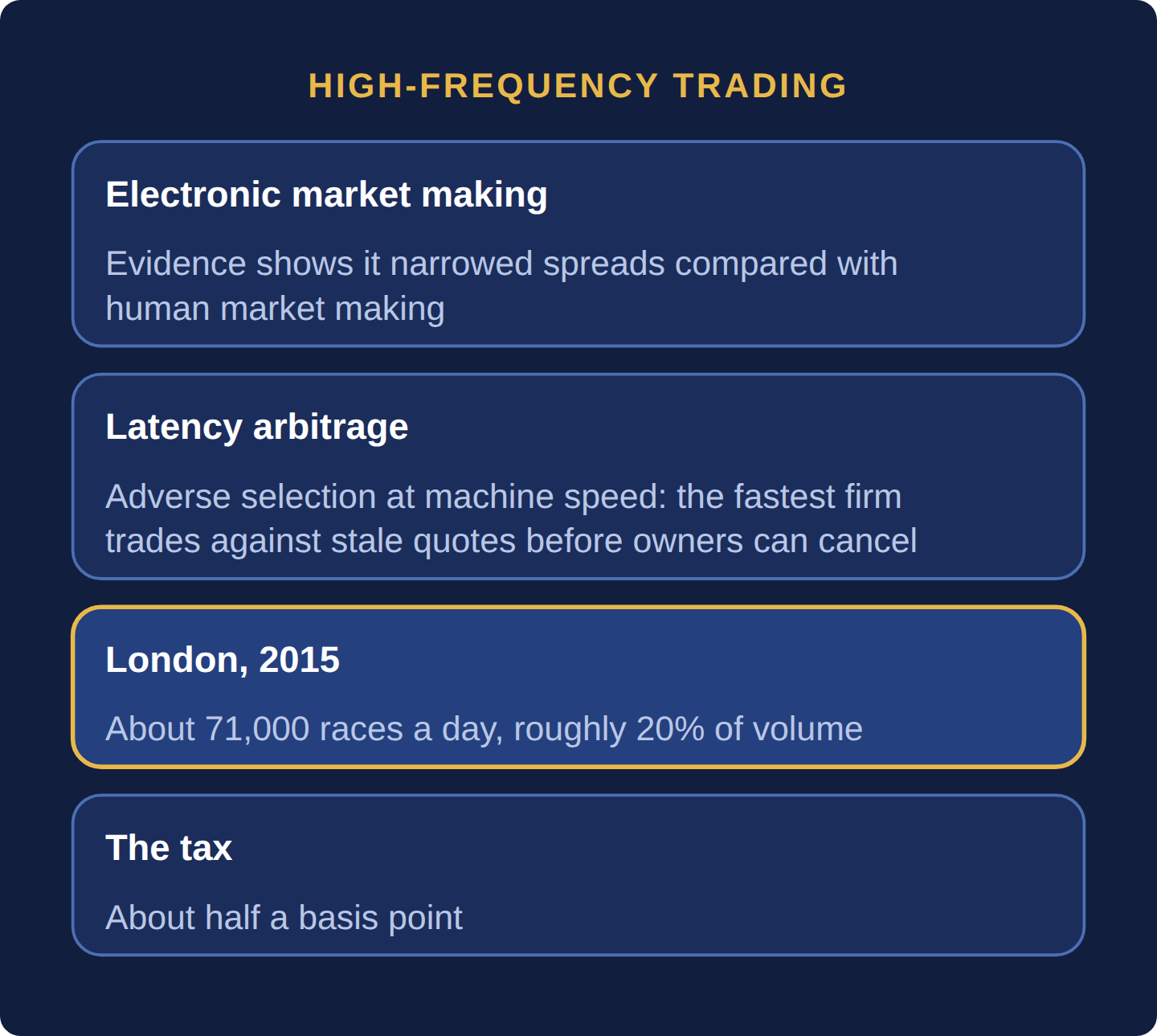
High-frequency trading (HFT), named in Capital Markets Part 8, captures its edge through genuine, measurable speed advantages operating at the microsecond and even nanosecond scale. Latency arbitrage exploits the tiny, real time delay between when a price changes on one exchange and when that same information becomes available and actionable on another exchange or trading venue — an HFT firm with a faster connection can react to the price change and trade on the slower venue before that venue’s own participants have even seen the update. This drove the specific practice of co-location: HFT firms paying substantial fees to place their own trading servers physically inside the same data center as an exchange’s own matching engine, minimizing the physical distance — and therefore the time — data must travel.
Latency arbitrage is adverse selection at machine speed. When news moves the price on one venue, every resting quote elsewhere is briefly stale, and the fastest firm can trade against it before its owner can cancel. A study of London Stock Exchange message data for FTSE 350 stocks in 2015 by Aquilina, Budish and O’Neill, NBER w29011 found about 71,000 such races a day, lasting a modal 5 to 10 microseconds, with 22% of FTSE 100 trading volume taking place in races. The races act like a tax of about half a basis point on trading volume (0.42 bps measured on all volume), account for about a third of price impact (31%), and sum to roughly $5 billion a year across global equity markets; removing them would cut investors’ cost of liquidity by an estimated 17%.
Imagine a horse race where the results are announced over two separate loudspeakers — one right next to the finish line, and one a mile away in town. Anyone standing right next to the finish line loudspeaker knows the result a fraction of a second before anyone in town does, and can place a bet with someone in town before news of the actual result reaches them. HFT’s speed edge works on exactly this principle, played out across financial markets in microseconds rather than seconds.
This speed race has driven heavy infrastructure spending. In the words of the London latency-race study above, it involves “microwave links between market centers, trans-oceanic fiber-optic cables, putting trading algorithms onto hardware as opposed to software, co-location rights and proprietary data feeds from exchanges.” On the critics’ view (below), each improvement pays mainly by beating rivals, so the spending repeats without serving investors.
HFT firms are also the main liquidity providers in modern markets: much of the electronic market making in Section 5.3: Market Makers and the Bid-Ask Spread is high-frequency. The same speed that lets a firm snipe stale quotes lets it update its own quotes quickly, which reduces the adverse selection it faces and lets it quote tighter. That is why the evidence on HFT points in two directions.
The case for: Hendershott, Jones and Menkveld (2011) used the NYSE’s 2003 move to automated quote dissemination as a natural experiment and found that, for large stocks, more algorithmic trading narrowed quoted and effective spreads, with most of the narrowing coming from lower adverse selection. Faster quoting firms take less risk, so they can quote tighter.
The case against: Budish, Cramton and Shim (2015) argue that in a continuous order book any public price move creates a race to snipe stale quotes, so speed investment is socially wasteful and its cost is passed to investors through wider spreads. The measured size of that tax (about 0.5 bps and $5 billion a year) comes from the London data cited above.
What remains open: both can be true: automation cut costs compared with human market making, while continuous trading leaves a residual tax. The live question is whether fixes such as frequent batch auctions are worth the cost of redesigning markets.
Speed also multiplies mistakes. When an algorithm misreads the market or a software release goes wrong, losses that once took a day accumulate in minutes. Two well-documented cases show why the price bands and pauses in Section 5.4: Price-Time Priority and Matching Engines and the pre-trade controls below exist.
The Flash Crash, May 6, 2010. According to the joint CFTC–SEC staff report on May 6, 2010, a large trader began selling 75,000 E-Mini S&P 500 futures contracts, worth about $4.1 billion, with an algorithm set to sell 9% of the previous minute’s volume “without regard to price or time.” It finished in about 20 minutes. Between 2:41 p.m. and 2:45:27 p.m. the E-Mini fell more than 5% as high-frequency traders passed contracts back and forth (the report’s “hot potato” volume), which the algorithm read as volume and sold into. A five-second pause at 2:45:28 p.m. let prices stabilize. In single stocks, more than 20,000 trades in over 300 securities executed 60% or more away from earlier prices, some at a penny against placeholder “stub quotes”; those trades were canceled. Lesson: an algorithm that targets volume but ignores price can feed on its own selling.
Knight Capital, August 1, 2012. A faulty deployment of new order-routing code, with old unused code still in the system, sent millions of orders in 45 minutes and produced over 4 million executions in 154 stocks for more than 397 million shares, according to the SEC order, In the Matter of Knight Capital Americas (2013). Knight ended up about $3.5 billion long in 80 stocks and $3.15 billion short in 74 others, and lost over $460 million, roughly $10 million a minute. The SEC fined it $12 million under the Market Access Rule (Rule 15c3-5, adopted 2010), which requires brokers with direct market access to have pre-trade risk controls. Operational-risk controls more broadly are the subject of Part 8: Operational Risk Governance & Reconciliation.
A reading rule for HFT claims: ask which activity is meant. For electronic market making, the evidence to check is spreads and depth; for latency arbitrage, it is the race tax on resting quotes. For anyone running an algorithm: if a strategy can send orders, it needs hard pre-trade limits on size, position and loss, and a kill switch a human can use in seconds. Monitoring alone is not enough; Knight received internal alert emails before the open.
Deploying trading code without tested pre-trade limits and a kill switch. Knight Capital lost over $460 million in 45 minutes, about $10.2 million a minute (460 ÷ 45). A limit that blocked new orders once gross exposure exceeded a set multiple of normal would likely have capped the losses within minutes. SEC Rule 15c3-5 requires such controls; having them on paper is not the same as testing them on every release.
How do high-frequency traders make money?
Mostly in two ways: market making, earning small spreads and exchange rebates on very large volume, and latency arbitrage, trading against stale quotes before their owners can cancel. Profits per trade are tiny; the London study found average race profits of about two pounds.
What caused the 2010 Flash Crash?
The joint CFTC–SEC report traced it to a $4.1 billion E-Mini sell program executed by an algorithm that targeted 9% of volume regardless of price, in an already stressed market. Fast traders passing contracts among themselves inflated volume, the algorithm sold faster, and single-stock liquidity collapsed.
Is co-location legal?
Yes. Exchanges in the US and India rent space beside their matching engines and must offer it on fair terms. The problem in India’s NSE case was not co-location itself but a data-feed design that let brokers who connected first see prices earlier (see the India Lens).
HFT’s edge is speed, used for electronic market making and for latency arbitrage against stale quotes, which London data price at about half a basis point of volume. The Flash Crash and Knight Capital show how fast algorithmic errors compound, which is why pre-trade limits and kill switches are mandatory.
Six questions on this chapter. Decide on your answer first, then click “Reveal Answer.”
1. Knight Capital lost over $460 million in 45 minutes. Roughly how much was that per minute?
- About $4.6 million
- About $10 million
- About $46 million
- About $1 million
Reveal Answer
Answer: B. 460 ÷ 45 ≈ $10.2 million a minute.
2. What is latency arbitrage?
- Routing orders to the venues with the lowest access fees
- Buying shares in one auction to sell them in the next one
- Trading against stale quotes before their owners can update them
- Earning rebates by posting the same quotes on many exchanges
Reveal Answer
Answer: C. When prices move, quotes elsewhere are briefly stale, and the fastest firm trades against them first.
3. What did Hendershott, Jones and Menkveld (2011) find about algorithmic trading in large NYSE stocks?
- It widened spreads, mainly by raising inventory costs
- It had no measurable effect on quoted spreads
- It raised trading fees charged to institutional investors
- It narrowed spreads, mainly by lowering adverse selection
Reveal Answer
Answer: D. Using the 2003 autoquote change, they found narrower quoted and effective spreads, most of it from lower adverse selection.
4. What feature of the 2010 sell algorithm contributed to the Flash Crash, according to the CFTC–SEC report?
- It targeted 9% of volume without regard to price or time
- It sold only when prices were above the prior day’s close
- It routed all of its orders to dark pools to hide size
- It split the order evenly across five days of trading
Reveal Answer
Answer: A. The algorithm sold faster as volume rose, including volume created by fast traders passing contracts among themselves.
5. Worked problem: Latency arbitrage costs about half a basis point of traded value. On $2bn of daily volume, what is the daily tax?
Reveal Answer
Answer: $2,000,000,000 × 0.00005 = $100,000 a day.
6. Worked problem: If 20% of volume is involved in such races, what is the cost of the races themselves, as a share of that volume?
Reveal Answer
Answer: The tax is spread across all volume at 0.5 bp, so on the raced 20% the cost is 0.5 bp ÷ 0.20 = 2.5 bps.
- SEC, In the Matter of Knight Capital Americas LLC (Release 34-70694, 2013) — Knight Capital executions, positions and loss
- CFTC and SEC staff, Findings Regarding the Market Events of May 6, 2010 — Flash Crash facts