
8.3 Macro and Event-Driven Strategies
A global macro fund trades big-picture views on interest rates, currencies and government risk. An event-driven fund trades specific corporate events, such as mergers and bankruptcies. In merger arbitrage, the gap between the offer price and the market price reflects the chance the deal falls through. So the trade is a small, likely gain against a large, unlikely loss, much like selling insurance.
Why it matters: A steady small profit can hide a rare, large loss.
Summary: Global macro funds trade top-down views on rates, currencies and sovereign risk; event-driven funds trade identifiable corporate events such as mergers and bankruptcies. In merger arbitrage the spread prices the chance the deal fails, so the trade is a small likely gain against a large unlikely loss, much like selling insurance.
- Spread = (deal value − price) ÷ price; 5.26% over six months is 10.8% a year compounded.
- Implied completion probability = (price − break price) ÷ (offer − break price): 79% before interest, 87% after, in the example.
- With your own 85/10/5 view the expected return is 3.26% in six months; the trade loses money on average above a 22.9% break probability.
- Mitchell and Pulvino (2001): about 4% a year of excess return, with payoffs like selling index puts.
- Capri fell 45% in a day when the FTC won its injunction in October 2024.

Global macro funds trade based on top-down views of entire economies and asset classes — interest rate direction, currency moves, sovereign risk — using instruments from across this Volume (bonds, currency swaps, index futures) rather than individual company analysis; this is the strategy behind famous macro trades like betting against a currency peg. Event-driven strategies instead trade around specific, identifiable corporate events: merger arbitrage (buying the target after a deal is announced, and in a stock-for-stock deal also shorting the acquirer, profiting from the spread between the current market price and the announced deal price, betting the deal closes as announced) and distressed debt investing (buying the bonds of a financially troubled company at a deep discount, betting on a favorable recovery through restructuring or bankruptcy).
The payoff is asymmetric: a small, likely gain (the spread) against a large, unlikely loss (the break). That is the payoff of an investor who sells a put option, collecting a premium in normal times and paying out in a crash, and deals are most likely to fail when markets fall, because financing dries up and buyers walk. Mitchell and Pulvino (Journal of Finance, 2001), studying 4,750 mergers from 1963 to 1998, found risk-arbitrage returns uncorrelated with the market in flat and rising markets but positively correlated in severely falling ones, “similar to those obtained from selling uncovered index put options”; after transaction costs and controlling for that nonlinearity, excess returns were about 4% a year. A global macro fund that holds long-volatility or short-risk positions can have the opposite profile in a sell-off, which is why allocators treat the two as complements rather than substitutes.
Merger arbitrage returns depend almost entirely on deal-completion risk, not overall market direction — the spread exists precisely because the market is pricing in some probability the deal falls through (due to financing failure, antitrust rejection, or a shareholder vote defeat), which is exactly why this strategy is often described as earning a steady, low-correlation return stream, punctuated by sharp losses on the rare occasions a deal actually breaks.
An acquirer offers $50.00 cash per share. The target traded at $38.00 before the announcement (its unaffected price) and now trades at $47.50; closing is expected in six months; the risk-free rate is 4%.
- Gross spread = (50.00 − 47.50) ÷ 47.50 = 5.26% for six months; annualized = 1.0526² − 1 = 10.8% (10.5% simple).
- Implied probability of completion = (price − break price) ÷ (offer − break price) = (47.50 − 38.00) ÷ (50.00 − 38.00) = 79.2%. Allowing for six months of interest, 47.50 × 1.02 = 48.45, so p = (48.45 − 38.00) ÷ 12.00 = 87.1%. The break price is where the stock would trade if the deal failed; the unaffected price is only a first guess, since the target’s sector may have moved since.
| Scenario (your probability) | Price at resolution | Return on $47.50 | Probability × payoff |
|---|---|---|---|
| Deal closes (85%) | $50.00 | +5.3% | 0.85 × 50.00 = 42.50 |
| Deal breaks (10%) | $38.00 | −20.0% | 0.10 × 38.00 = 3.80 |
| Topping bid (5%) | $55.00 | +15.8% | 0.05 × 55.00 = 2.75 |
| Expected value | $49.05 | +3.26% in six months | vs 2.0% risk-free |
The flip point. Holding the topping-bid chance at 5%, the expected value falls by $12.00 for each unit of break probability moved from “closes” to “breaks”. The trade earns only the risk-free rate when (0.95 × 50.00 + 0.05 × 55.00 − 48.45) ÷ 12.00 = 15.0% break probability, and loses money on average above (0.95 × 50.00 + 0.05 × 55.00 − 47.50) ÷ 12.00 = 22.9%. One break costs $9.50 a share, the spread of 3.8 completed deals.
A real break. On October 24, 2024, a federal judge granted the FTC’s injunction against Tapestry’s $57-a-share, $8.5 billion purchase of Capri; the next day Capri fell 45%, to $22.82. Working back, the pre-ruling price was about 22.82 ÷ 0.55 = $41.49, which priced completion at only (41.49 − 22.82) ÷ (57.00 − 22.82) = 55%. The market had seen the antitrust risk; anyone who sized the position on the 37% upside alone lost 45%.
Never judge a deal by its annualized spread alone. Estimate the break price, compute the market’s implied completion probability after interest, and enter only if your own probability, built from antitrust overlap, financing, shareholder vote and regulatory timetable, is clearly higher (as a heuristic, at least 5 percentage points). Size the position so that a break, a loss of several times the spread (3.8 times in the example), costs no more than about 1% to 2% of the portfolio. Re-run the arithmetic whenever the expected closing date slips: a six-month spread that takes twelve months halves its annualized return.
Treating the spread as a bond yield. A 10.8% annualized spread looks like high-yield income, but its downside is equity-like: in the example one break loses $9.50, the gain from 3.8 completed deals, and in the Capri case a 37% expected gain turned into a 45% loss in a day. Concentrating in a few large, antitrust-sensitive deals, or levering the book because the realized volatility was low, turns a steady strategy into a single bet on a court ruling.
How do you calculate a merger arbitrage spread?
Spread = (deal value − current target price) ÷ current target price. For a cash deal the deal value is the offer price; for a stock deal it is the exchange ratio times the acquirer’s price. Annualize it over the expected time to close: 5.26% in six months is 10.8% a year compounded.
What does the spread tell you about the odds of a deal closing?
The implied probability is (target price − break price) ÷ (deal value − break price), adjusted for interest. A $47.50 price between a $50.00 offer and a $38.00 break price implies about 79% before interest and 87% after. The estimate is only as good as the break price you assume.
What is distressed debt investing?
Buying the bonds or loans of a company in or near default at a deep discount, betting that the recovery in a restructuring or bankruptcy will exceed the price paid. A bond bought at 40 cents that recovers 55 cents in two years returns 37.5%, about 17% a year; one that recovers 25 cents loses 37.5%.
Macro funds trade top-down views; event-driven funds trade mergers and distress. A merger spread prices deal risk: compute the annualized spread, estimate the break price, back out the implied completion probability, and size the position so that a break, worth several completed deals, is survivable.
Six questions on this chapter. Decide on your answer first, then click “Reveal Answer.”
1. A target trades at $28.50 against a $30.00 all-cash offer, and the deal is expected to close in four months. What is the annualized (compounded) spread?
- About 10.8%
- About 5.3%
- About 16.6%
- About 15.8%
Reveal Answer
Answer: C. Spread = (30.00 − 28.50) ÷ 28.50 = 5.26% for four months; (1.0526)³ − 1 = 16.6%. 15.8% is the simple annualization and 5.3% the unannualized spread.
2. Same deal: if the deal fails, you expect the target to trade at $22.00. Ignoring interest, what completion probability does the market price imply?
- About 81%
- About 73%
- About 95%
- About 87%
Reveal Answer
Answer: A. Implied probability = (price − break price) ÷ (offer − break price) = (28.50 − 22.00) ÷ (30.00 − 22.00) = 6.50 ÷ 8.00 = 81.25%.
3. Why do Mitchell and Pulvino (2001) compare risk-arbitrage returns to selling uncovered index put options?
- Arbitrageurs buy index puts to hedge each deal against a fall in the market
- Returns are uncorrelated with stocks in calm markets but fall with them in severe declines
- Returns rise most when the stock market falls sharply, like a protective put
- Spreads are priced off index option implied volatility, like an insurance premium
Reveal Answer
Answer: B. Like a put writer, the arbitrageur collects small gains most of the time and suffers large losses when markets crash, because deals fail more often in sell-offs.
4. A distressed bond is bought at 50 cents on the dollar and recovers 65 cents in a restructuring two years later. What is the annualized return?
- About 13.0%
- About 30.0%
- About 15.0%
- About 14.0%
Reveal Answer
Answer: D. Total return is 65 ÷ 50 − 1 = 30%; annualized over two years, √1.30 − 1 = 14.0%. 15.0% simply halves the total.
5. Worked problem: A target trades at $47 and the deal price is $50. What is the spread, and annualized if the deal closes in four months?
Reveal Answer
Answer: Spread = $50 ÷ $47 − 1 = 6.38%. Annualized = (1 + 0.0638)3 − 1 = 20.4%.
6. Worked problem: If the stock would fall to $35 if the deal broke, what completion probability does the price imply (before interest)?
Reveal Answer
Answer: p = (price − break) ÷ (offer − break) = (47 − 35) ÷ (50 − 35) = 80%.
8.4 Quantitative Strategies
Quantitative strategies follow systematic rules at large scale, from pairs trades and statistical arbitrage to high-frequency market making. Their edge comes from making many small, independent bets, like a casino earning a little on every hand. Whether that edge survives depends on trading costs and on how crowded the strategy has become.
Why it matters: An edge that many people copy, or that costs too much to trade, disappears.
Summary: Quantitative strategies apply systematic rules at scale, from pairs trades and statistical arbitrage to high-frequency market making. Their edge comes from many small, independent bets, and trading costs and crowding decide whether that edge survives.
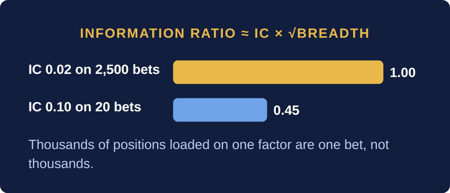
- Fundamental law: information ratio ≈ IC × √breadth; IC 0.02 on 2,500 bets beats IC 0.10 on 20.
- Thousands of positions loaded on one factor are one bet, not thousands.
- At 200 trades a year, one extra basis point of cost halves a 4% net return.
- A pairs trade enters on a z-score near 2 and should be cut, not doubled, if the spread breaks far beyond its history.
- August 2007 showed crowded, levered quant books unwinding together.
Quant strategies use systematic, model-driven rules — often built on the factor models from Part 5: Portfolio Theory & Quant Risk — to make investment decisions at scale, largely removing discretionary human judgment from individual trade decisions. Statistical arbitrage identifies temporary pricing anomalies between historically related securities, betting on their eventual convergence back to a normal relationship. High-frequency trading (HFT) operates on a vastly shorter time horizon, using speed and technology advantages to capture very small, very frequent pricing inefficiencies, often holding positions for mere seconds.
A pairs trade is the simplest statistical arbitrage. Regress stock A’s price on stock B’s to estimate a hedge ratio, say 1.5, and track the spread A − 1.5 × B. If the spread has averaged $0 with a standard deviation of $1.20 and now stands at $2.70, its z-score (Section 0.4: The Quant Toolkit) is 2.70 ÷ 1.20 = 2.25: the model sells A and buys 1.5 shares of B for each share of A, and closes when the spread returns toward zero. The risk is that the relationship has broken for a reason, a takeover or a fraud, rather than drifted by chance.
Grinold’s “fundamental law of active management” (Journal of Portfolio Management, 1989) approximates a manager’s information ratio (active return per unit of active risk, Part 5.4: The Sharpe Ratio & Risk-Adjusted Return) as IR ≈ IC × √breadth, where the information coefficient (IC) is the correlation between forecasts and outcomes and breadth is the number of independent bets a year. A discretionary manager with an IC of 0.10 on 20 independent bets gets 0.10 × √20 = 0.45. A quant whose signal is barely better than chance, IC 0.02, applied to 2,500 independent bets gets 0.02 × √2,500 = 1.00. Breadth beats insight, but only if the bets are truly independent: thousands of positions all loaded on the same value or momentum factor are one bet, not thousands.
Costs decide the rest. A strategy that earns 6 basis points per round trip before costs, trades 200 times a year and pays 4 basis points per round trip makes 200 × 6 = 12% gross, 200 × 4 = 8% in costs and 4% net. One more basis point of cost (market impact rises as the fund grows) halves the net return to 2%. This is why capacity, not ideas, limits most quant funds, and why high-frequency traders invest in speed: at holding periods of seconds, the edge per trade is a fraction of a cent and costs are everything.
Back a systematic signal only if its expected edge per trade is at least twice its all-in trading cost (commission, spread and market impact at the intended size), its backtest survives out-of-sample data the designer did not see, and its positions are not the same factor bet under another name. If a pairs spread moves beyond about 4 standard deviations, assume the relationship may have broken and cut the position rather than adding to it; the 2-standard-deviation entry rule assumes the past distribution still holds.
Running a crowded strategy with leverage. In the week of August 6, 2007, many quantitative long/short equity funds suffered what Khandani and Lo (2008) called “unprecedented losses”: similar portfolios, typically long cheap stocks (high book-to-market) and short those with strong earnings momentum, were unwound together as funds deleveraged, and market makers withdrew risk capital from August 8. Each fund’s diversification was an illusion because its neighbors held the same trades. Measure your overlap with common factor portfolios, keep leverage low enough to survive a multi-standard-deviation week, and do not assume you can exit at model prices when everyone with your model is selling.
What is statistical arbitrage?
A family of systematic strategies that bet on the convergence of prices that have historically moved together, from single pairs to portfolios of thousands of stocks. It is not arbitrage in the riskless sense: convergence is likely, not guaranteed, and the spread can widen far beyond the model’s range before it closes.
Is high-frequency trading the same as quant investing?
No. HFT firms mostly make markets and exploit tiny, fleeting price differences, holding positions for seconds and ending the day flat; their edge is speed and cost. Quant investment funds hold positions for days to months based on factor and statistical models. Both are systematic, but they compete on different things.
Why do quant strategies stop working?
Because returns attract capital, and capital raises trading costs and crowds the signal. Some backtested signals were also never real: test enough variables and some will look profitable by chance, which is why out-of-sample testing matters.
Quant strategies rely on breadth: a small edge applied to many independent bets can produce a high information ratio. Trading costs, capacity and crowding decide whether that edge survives, as the August 2007 quant unwind showed.
Six questions on this chapter. Decide on your answer first, then click “Reveal Answer.”
1. Under Grinold’s fundamental law, what information ratio does a signal with an information coefficient of 0.05 applied to 400 independent bets a year imply?
- About 20
- About 0.5
- About 0.25
- About 1.0
Reveal Answer
Answer: D. IR ≈ IC × √breadth = 0.05 × √400 = 0.05 × 20 = 1.0. 20 forgets the square root; 0.5 uses 100 bets.
2. A strategy earns 8 basis points per round trip before costs, trades 150 times a year and pays 5 basis points per round trip. What is its net annual return?
- 4.5%
- 3.0%
- 12.0%
- 7.5%
Reveal Answer
Answer: A. Gross 150 × 8 bp = 12.0%; costs 150 × 5 bp = 7.5%; net 4.5%. Small changes in cost per trade swing the net result heavily.
3. According to Khandani and Lo, what drove the quant losses in the week of August 6, 2007?
- A trading-system failure at one large high-frequency firm that spread to others
- Forced unwinding of similar long/short portfolios, then market makers pulling back
- Fraudulent valuations at funds holding illiquid loans, which forced redemptions
- A surprise Federal Reserve rate hike that hit value stocks the hardest
Reveal Answer
Answer: B. Many funds held similar positions (long high book-to-market, short earnings momentum); deleveraging by some hit all of them, and market makers withdrew risk capital from August 8.
4. A pairs spread has averaged $0 with a standard deviation of $1.50 and now stands at $3.00. What is its z-score, and what does the model do?
- 2.0; buy both legs and hold them together
- 4.5; add to both legs and widen the position
- 2.0; sell the rich leg and buy the cheap one
- 0.5; take no position until the spread reverts
Reveal Answer
Answer: C. z = 3.00 ÷ 1.50 = 2.0, a typical entry threshold: the model shorts the leg that is rich relative to the hedge ratio and buys the other, betting on convergence.
5. Worked problem: A manager has an information coefficient of 0.05 and makes 400 independent bets a year. What information ratio does the fundamental law give?
Reveal Answer
Answer: IR ≈ IC × √breadth = 0.05 × √400 = 1.00.
6. Worked problem: Another manager has IC 0.10 but only 25 bets. Who has the higher ratio?
Reveal Answer
Answer: IR = 0.10 × √25 = 0.50, half the first manager’s. Breadth beats skill per bet.
- Grinold (1989), The Fundamental Law of Active Management, The Journal of Portfolio Management — The fundamental law linking skill, breadth and the information ratio
- Fama & French (1993), Common risk factors in the returns on stocks and bonds, Journal of Financial Economics — The three-factor model behind many quantitative strategies