
5.1 Diversification — Why Combining Assets Reduces Risk
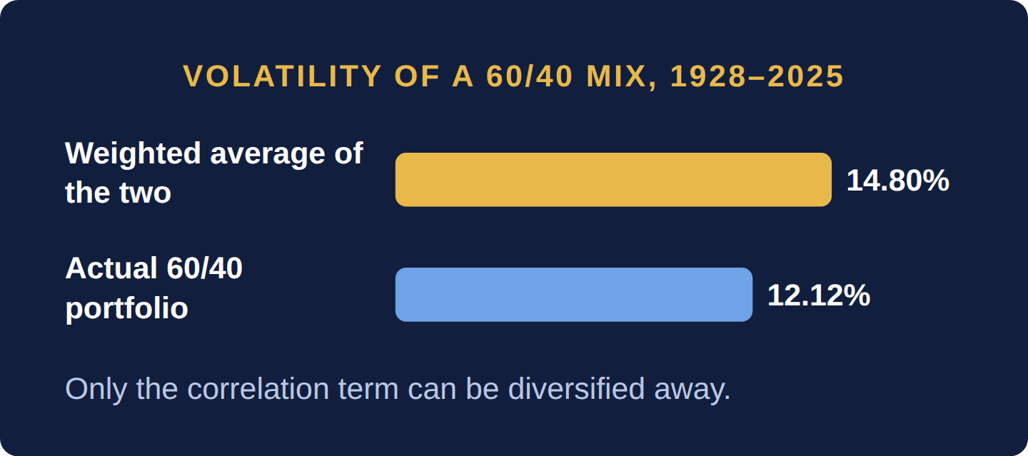
Diversification lowers risk because a portfolio’s ups and downs depend on how its parts move together, not only on how wild each part is. It is like not putting all your eggs in one basket, and choosing baskets that don’t drop at the same time. US data for 1928 to 2025 show a 60/40 mix of stocks and bonds had 12.12% volatility, against a 14.80% weighted average of the two, with no loss of expected return. The benefit shrinks as the parts move more alike, and can vanish in a crisis when stocks and bonds fall together.
Why it matters: Diversification is about as close to a free benefit as investing offers, but it can fail in a crisis.
Summary: Diversification lowers risk because a portfolio’s variance depends on how its assets move together, not only on how volatile each one is. With US data for 1928–2025, a 60/40 stock–bond mix had 12.12% volatility against a 14.80% weighted average, with no loss of expected return. The benefit shrinks as correlation rises and vanishes in a crisis if stocks and bonds fall together.
- Two-asset variance: σp² = w₁²σ₁² + w₂²σ₂² + 2w₁w₂ρσ₁σ₂; only the correlation term can be diversified.
- Adding stocks removes idiosyncratic risk but leaves a floor of systematic (market) risk.
- The stock–bond correlation was −0.65 over 2000–2021 and +0.88 over 2022–2025; the 60/40 benefit fell from 4.92 to 0.30 points.
- Flip point: stocks lower an all-bond portfolio’s risk only while ρ is below σbond ÷ σstock ≈ 0.41.
- Judge diversification by correlation under stress, not by the number of holdings.
Volume I introduced insurers and pension funds as institutions managing very large pools of capital. This Part asks the mathematical question underneath their entire discipline: given a universe of assets, each with its own expected return and risk, how should capital actually be allocated among them?
The foundational insight, formalized by Harry Markowitz in 1952, is that a portfolio’s total risk depends not just on the risk of each individual asset, but on how those assets move relative to one another — their correlation. Combining two assets that are not perfectly correlated reduces the portfolio’s overall volatility below the simple average of the two assets’ individual volatilities, without necessarily sacrificing any expected return. This is diversification’s free lunch: a benefit that costs nothing in expected return, available purely from combining imperfectly correlated assets, for as long as the correlation stays low.
Imagine two street vendors in the same market: one sells umbrellas, one sells sunglasses. Each vendor’s daily income is individually volatile — heavily dependent on the day’s weather. But their combined income is far steadier than either one alone, because rain that hurts sunglasses sales helps umbrella sales, and vice versa. Their businesses are negatively correlated, and that negative correlation — not any change in either business individually — is what smooths the combined outcome.
For two assets with weights w₁ and w₂, volatilities σ₁ and σ₂ and correlation ρ (the statistics are reviewed in Section 0.4: The Quant Toolkit), portfolio variance is:
σp² = w₁²σ₁² + w₂²σ₂² + 2w₁w₂ρσ₁σ₂
Only the third term depends on how the assets move together, and it is the only term diversification can shrink. US annual returns for 1928–2025 give the inputs: stocks (S&P 500 with dividends) averaged 11.85% with σ = 19.40%; 10-year Treasury bonds averaged 4.82% with σ = 7.90%; their correlation was +0.02. For a 60/40 mix:
σp² = 0.6² × 0.1940² + 0.4² × 0.0790² + 2 × 0.6 × 0.4 × 0.02 × 0.1940 × 0.0790 = 0.013549 + 0.000999 + 0.000147 = 0.014695, so σp = √0.014695 = 12.12%.
The weighted average of the two volatilities is 0.6 × 19.40% + 0.4 × 7.90% = 14.80%. The 2.68-point gap is the diversification benefit, while expected return stays at 0.6 × 11.85% + 0.4 × 4.82% = 9.04% whatever the correlation.
The same algebra explains why adding stocks stops helping. With N equal-weighted stocks, each with σ = 35% and an average pairwise correlation of 0.25 (illustrative), portfolio volatility is 35% × √(1/N + (1 − 1/N) × 0.25): 19.95% at N = 10, 18.35% at N = 30, and a floor of 35% × √0.25 = 17.5% however many stocks you add. That floor is systematic risk; the part that disappears is idiosyncratic risk, and only systematic risk earns a premium under CAPM (Section 1.5: CAPM — The Cost of Equity).
The stock–bond correlation is not a constant. In the same dataset it was −0.65 over 2000–2021 and +0.88 over 2022–2025 (only four annual observations, so read it as a stress reading, not an estimate). Everything else is held at the inputs above.
| Correlation regime | 60/40 volatility | Benefit vs. 14.80% average | Minimum-variance stock weight | Lowest attainable volatility |
|---|---|---|---|---|
| −0.65 (2000–2021) | 9.88% | 4.92 points | 25.4% | 4.61% |
| +0.02 (1928–2025) | 12.12% | 2.68 points | 13.7% | 7.37% |
| +0.88 (2022–2025) | 14.50% | 0.30 points | 0% (all bonds) | 7.90% |
Flip point. Adding a little stock to an all-bond portfolio lowers its risk only while ρ < σbond ÷ σstock = 7.90% ÷ 19.40% = 0.41. Above 0.41 the riskier asset stops hedging the safer one and only adds volatility. In 2022 US stocks returned −18.0% and 10-year Treasuries −17.8% in this dataset: the year the 60/40 hedge failed.
Judge diversification by correlation, not by the count of holdings. Compute portfolio volatility twice: with the long-run correlation and with a stressed one (the highest rolling one-year correlation in your data, or +0.8 when the history is short). If the stressed volatility is within about one percentage point of the weighted-average volatility, assume the diversification will be absent when you need it, and add an asset with a different economic driver rather than more names with the same one. Beyond roughly 20 to 30 stocks with similar exposures, extra names barely move the floor. Do not apply the rule to illiquid assets whose low measured correlation comes from stale appraisal prices.
Counting names instead of correlations. Thirty technology stocks with an average correlation of 0.6 (illustrative, σ = 35% each) give 35% × √(1/30 + 29/30 × 0.6) = 27.41% volatility, against 18.35% for thirty stocks at 0.25: 49% more risk behind a holdings list that looks just as diversified. On a $1 million portfolio, a two-standard-deviation bad year is then about $548,000 instead of $367,000 (ignoring expected return). Avoid it by grouping holdings by what drives them, then sizing the groups.
How many stocks do you need to be diversified?
About 20 to 30 stocks with different business drivers remove most idiosyncratic risk, and the gain beyond that is small. In the illustration above, going from 10 to 30 stocks cuts volatility from 19.95% to 18.35%, and even infinite holdings only reach 17.5%. What no number of stocks removes is market risk, which is why a 500-stock index fund still lost 18.0% in 2022.
Is diversification really a free lunch?
It is free in expected return, not free in every state of the world. Mixing assets lowers volatility without lowering the weighted-average expected return, but the size of the benefit depends on correlation, and correlations tend to rise in crises. In the 60/40 example the benefit falls from 2.68 points to 0.30 points when the stock–bond correlation moves from 0.02 to 0.88.
Do bonds always hedge stocks?
No. US stock and Treasury returns were negatively correlated over 2000–2021 (−0.65 in annual data), so bonds cushioned equity losses, as in 2008 when stocks lost 36.6% and Treasuries gained 20.1%. When inflation and rising rates drive both, as in 2022, both fall together. Bonds hedge growth scares well and inflation shocks badly.
Portfolio risk depends on correlation as well as on each asset’s volatility: with 1928–2025 US data, a 60/40 mix had 12.12% volatility against a 14.80% weighted average. Adding stocks removes idiosyncratic risk but not systematic risk, and the stock–bond diversification benefit fell from 4.92 to 0.30 points as correlation moved from −0.65 to +0.88, so test diversification under stressed correlations.
Six questions on this chapter. Decide on your answer first, then click “Reveal Answer.”
1. A portfolio holds 50% stocks (σ 20%) and 50% bonds (σ 10%) with a correlation of 0.5. What is its volatility?
- About 11.2%
- About 13.2%
- About 9.4%
- About 15.0%
Reveal Answer
Answer: B. σp² = 0.25 × 0.04 + 0.25 × 0.01 + 2 × 0.25 × 0.5 × 0.20 × 0.10 = 0.0175, and √0.0175 = 13.2%. 15.0% is the weighted average, which would require a correlation of 1; 11.2% ignores the covariance term.
2. Which part of a stock portfolio’s risk remains however many similar stocks you add?
- Liquidity risk from trading many small positions
- Idiosyncratic risk specific to each company
- Systematic risk shared by all of the stocks
- Currency risk from foreign-listed share classes
Reveal Answer
Answer: C. With N stocks, variance approaches the average covariance, which sets a floor (17.5% in the chapter’s illustration). Company-specific risk averages away.
3. Using the 1928–2025 volatilities (stocks 19.40%, bonds 7.90%), above roughly what correlation does adding a little stock to an all-bond portfolio stop reducing its risk?
- About 0.41
- About 0.88
- About 0.02
- Exactly 1.00
Reveal Answer
Answer: A. The flip point is ρ = σbond ÷ σstock = 7.90% ÷ 19.40% = 0.41. Below it, the covariance offset outweighs the added stock variance.
4. An investor holds 30 large technology stocks and says her portfolio is fully diversified. What is the best response?
- Diversification starts to work only once a portfolio holds at least 100 stocks
- Only adding government bonds can reduce the risk of any stock portfolio
- Thirty holdings remove nearly all risk regardless of which sectors they come from
- Correlated businesses keep her volatility far above a broad portfolio’s
Reveal Answer
Answer: D. At an average correlation of 0.6, thirty stocks with 35% volatility give 27.41% portfolio volatility, against 18.35% at 0.25. Correlation, not count, sets the risk.
5. Worked problem: A 50/50 portfolio holds assets with volatilities of 20% and 10% and a correlation of 0.30. What is its volatility?
Reveal Answer
Answer: Variance = 0.25 × 0.04 + 0.25 × 0.01 + 2 × 0.25 × 0.30 × 0.20 × 0.10 = 0.0155, so volatility = 12.45%.
6. Worked problem: Recompute it for correlations of +1.0 and −0.2. How much does diversification remove?
Reveal Answer
Answer: At ρ = 1 volatility is 15.00% (the weighted average, no diversification). At ρ = −0.2 it is 10.25%.
5.2 Modern Portfolio Theory & the Efficient Frontier
The efficient frontier is a menu of the best possible portfolios: for each level of risk, the one with the highest expected return. For US stocks and bonds over 1928 to 2025, the safest mix holds 13.7% stocks and has 7.37% volatility, and the frontier runs from there up to 100% stocks. Any portfolio below the frontier is beaten by another mix of the same assets. In practice, the optimizer that draws it magnifies mistakes in your return estimates, so professionals use it with limits.
Why it matters: The theory shows what is possible, but the inputs decide whether the answer is useful.
Summary: The efficient frontier is the set of portfolios with the highest expected return for each level of volatility. For US stocks and bonds over 1928–2025 it starts at a minimum-variance mix of 13.7% stocks (7.37% volatility) and runs to 100% stocks; anything below it is beaten by another mix of the same assets. In practice the optimizer behind it magnifies errors in expected-return estimates, so it is used with constraints.
- Minimum-variance weight: w* = (σB² − ρσSσB) ÷ (σS² + σB² − 2ρσSσB) = 13.7% stocks in the example.
- All bonds is inefficient: more risk and less return than the 13.7% stock mix.
- With 98 years of data, the 95% confidence interval on the stock mean is ±3.84 points.
- Moving the bond mean within its own confidence interval swings the optimal stock weight from 119% to 32%.
- Constrain weights and test sensitivity before implementing any optimized allocation.

Modern Portfolio Theory (MPT) extends this insight into a full framework: for any given level of risk (measured as the standard deviation of returns), there exists one combination of assets that delivers the highest possible expected return; equivalently, for any given target return, there exists one combination that achieves it with the lowest possible risk. Plotting every one of these optimal combinations across all possible risk levels traces a curve called the efficient frontier. Any portfolio sitting below this curve is, by definition, suboptimal — a portfolio-construction error, since some other combination of the same assets could deliver more return for the same risk, or the same return for less risk.
Inputs from Section 5.1: Diversification — Why Combining Assets Reduces Risk: stocks 11.85% (σ 19.40%), bonds 4.82% (σ 7.90%), correlation 0.02; cash, the 3-month Treasury bill, averaged 3.41% over the same 1928–2025 period. Each row is one mix.
| Stock weight | Expected return | Volatility | Sharpe ratio (Section 5.4: The Sharpe Ratio & Risk-Adjusted Return) |
|---|---|---|---|
| 0% | 4.82% | 7.90% | 0.18 |
| 13.7% (minimum variance) | 5.78% | 7.37% | 0.32 |
| 20% | 6.23% | 7.48% | 0.38 |
| 40% | 7.63% | 9.17% | 0.46 |
| 60% | 9.04% | 12.12% | 0.46 |
| 80% | 10.44% | 15.63% | 0.45 |
| 100% | 11.85% | 19.40% | 0.44 |
The minimum-variance portfolio weight is w* = (σB² − ρσSσB) ÷ (σS² + σB² − 2ρσSσB) = (0.006241 − 0.000307) ÷ (0.037636 + 0.006241 − 0.000613) = 0.005934 ÷ 0.043264 = 13.7% in stocks. Every mix with less stock than that is inefficient: all bonds carries more risk (7.90%) and less return (4.82%) than the 13.7% mix (7.37%, 5.78%). The efficient frontier is the upper branch from 13.7% to 100% stocks. Where you sit on it is a risk-tolerance choice, not an optimization output; Section 5.3: The Capital Market Line & the Market Portfolio shows how adding cash changes the choice.
The efficient frontier is the mathematical justification for the entire asset-allocation industry: a portfolio manager’s core job is not picking individual winning stocks, but constructing a combination of assets that sits as close to this frontier as possible for the client’s chosen risk level. This is precisely why large pension funds and insurers (Volume I’s Part 3) devote enormous resources to asset-allocation modeling rather than only individual security selection.
Markowitz’s optimizer treats expected returns as known. They are estimates. The standard error of a mean is σ ÷ √n (Section 0.4: The Quant Toolkit): for 98 years of stock returns, 19.40% ÷ √98 = 1.96%, so a 95% confidence interval on the 11.85% mean is ±3.84 points; for bonds it is 1.96 × 7.90% ÷ √98 = ±1.56 points. Feed the optimizer the two ends of the bond interval (3.26% and 6.38%) and the stock weight of the highest-Sharpe portfolio (Section 5.3: The Capital Market Line & the Market Portfolio) swings from 119% (with a 19% short position in bonds) to 32%, although the data cannot tell the two inputs apart. Michaud (1989) described the problem as mean-variance optimization’s “tendency to maximize the effects of errors in the input assumptions.” Practitioners respond with weight limits, by shrinking expected returns toward market-implied values, or by targeting minimum variance, which needs no return forecast at all.
If you use an optimizer, test it before trusting it: shift each expected return by one standard error (σ ÷ √years) and rerun. If any weight moves by more than about 20 percentage points, the inputs are driving the answer, so cap weights (for example, no asset class above 60%) or fall back to the minimum-variance or a fixed policy mix. Pick your point on the frontier from the loss you can tolerate in a bad year, then check it against the frontier rather than the reverse. The test matters less when cash flows are contractually fixed, as in a bond portfolio matched to known liabilities (Section 3.2: Duration — Measuring Interest Rate Sensitivity).
Treating historical averages as forecasts and optimizing without limits. With the 98-year data above, a bond expected return of 3.26% produces a 119% stock, −19% bond portfolio; 6.38% produces 32% stocks. Run both through 2008, when stocks returned −36.6% and Treasuries +20.1%: 1.19 × (−36.6%) − 0.19 × 20.1% = −47.3%, against 0.32 × (−36.6%) + 0.68 × 20.1% = +2.0%. A 49-point difference came from an input no one could estimate more precisely. Constrain weights and test sensitivity before you implement.
What is the efficient frontier in simple terms?
It is the set of portfolios that give the highest expected return for each level of volatility. Any mix below it is beaten by another mix of the same assets. In the stock–bond example the frontier runs from 13.7% stocks (7.37% volatility, 5.78% expected return) up to 100% stocks (19.40%, 11.85%); mixes with less than 13.7% stocks lie below it.
Does mean-variance optimization work in practice?
As a framework, yes; as an exact recipe, only with constraints. Expected returns are estimated with errors of several percentage points, and an unconstrained optimizer piles into whatever input happens to be overstated. Institutions use it with weight limits, return forecasts shrunk toward market-implied values, and sensitivity tests, and many rely on minimum-variance or policy mixes that need fewer forecasts.
Why can adding a risky asset lower total risk?
Because the covariance term can offset more than the asset’s own variance adds. Starting from all bonds, moving 13.7% into stocks lowers volatility from 7.90% to 7.37% while raising expected return, since the near-zero correlation means stock and bond swings partly cancel. This works only while the correlation is below the 0.41 flip point computed in Section 5.1: Diversification — Why Combining Assets Reduces Risk.
The efficient frontier runs from the minimum-variance portfolio (13.7% stocks, 7.37% volatility in the US example) to the highest-return asset; mixes below it are beaten by another mix of the same assets. Because expected returns are estimated with large errors, unconstrained optimizers swing wildly, so practitioners cap weights and test sensitivity.
Six questions on this chapter. Decide on your answer first, then click “Reveal Answer.”
1. Two uncorrelated assets have volatilities of 20% (A) and 10% (B). What weight in A gives the minimum-variance portfolio?
- 80%
- 50%
- 33%
- 20%
Reveal Answer
Answer: D. With ρ = 0, w* = σB² ÷ (σA² + σB²) = 0.01 ÷ 0.05 = 20%. The riskier asset still earns a place because it partly offsets the other.
2. In the chapter’s US stock–bond example, why is a 100% bond portfolio inefficient?
- A 13.7% stock mix has lower volatility and a higher expected return
- Bonds earned no return above Treasury bills across the 1928–2025 data
- Its Sharpe ratio was negative over the full 1928–2025 sample
- It sits exactly on the minimum-variance point of the curve
Reveal Answer
Answer: A. The 13.7% stock mix has 7.37% volatility and a 5.78% expected return, against 7.90% and 4.82% for all bonds, so all bonds lies below the frontier.
3. What problem did Richard Michaud (1989) identify in mean-variance optimization?
- It cannot be applied to any portfolio holding more than two assets
- It tends to maximize the effects of errors in the input assumptions
- It ignores the correlations between the asset classes it combines
- It always recommends equal weights whatever expected returns it is given
Reveal Answer
Answer: B. Small errors in expected returns produce large swings in optimal weights, which is why practitioners add constraints and sensitivity tests.
4. Shifting one expected return by a single standard error moves an optimizer’s stock weight by 40 points. What does the chapter’s decision rule suggest?
- Implement the new weights because the optimizer has found the true optimum
- Drop whichever asset has the largest standard error from the analysis
- Cap the weights or fall back to a minimum-variance or policy mix
- Raise the expected return further until the weights stop moving
Reveal Answer
Answer: C. A move above about 20 points means the inputs, not the data, are driving the answer, so the output should be constrained rather than trusted.
5. Worked problem: Stocks have 18% volatility, bonds 6% and their correlation is 0.20. What stock weight minimizes portfolio variance?
Reveal Answer
Answer: w* = (σB² − ρσSσB) ÷ (σS² + σB² − 2ρσSσB) = (0.0036 − 0.00216) ÷ 0.03168 = 4.5% stocks.
6. Worked problem: What is the volatility of that minimum-variance portfolio, and why is it below the bond-only volatility?
Reveal Answer
Answer: Volatility = 5.95%, below the 6.00% of an all-bond portfolio, because a little of the less correlated stock reduces risk.
- Markowitz (1952), Portfolio Selection, The Journal of Finance — The paper that introduced portfolio selection and diversification
- Michaud, “The Markowitz Optimization Enigma: Is ‘Optimized’ Optimal?”, Financial Analysts Journal, 1989 — Optimizers maximize the effects of input errors (5.2).